1 Introduction
The aim of this article works as the preamble to Bayesian statistics and demonstrates how Bayesian statistics can be applied to solve Pattern Recognition and Machine Learning (ML) problems. In fact, Bayesian statistics is an alternative probabilistic approach aside from Frequentist approach to construct statistical models based on Bayes’ Theorem. Specifically, similar to Frequentist approach, models in the sense of Bayesian are also assumed to follow some mathematical well-founded distributions, but the main difference is that instead of inferring point estimates for model parameters, Bayesian approach infers the distribution over model parameters, which gives extra information about the uncertainty of the estimated model parameters. About the main content, it is about using Bayesian statistics to learn Linear Regression model, which includes stating the assumptions about the data and model parameters; evaluating the distribution of model parameters as well as the predictive distribution for unseen data given training data; choosing the appropriate model via Bayesian Model Comparison; extracting effective parameters among myriad of parameters. Last but not least, this article also introduces some of the approximation methods for computing analytically-intractable distributions (i.e., distributions do not have closed-form solution and intractable to compute by hand), which includes Metropolis Hasting, Gibbs Sampling, Variational Inference, and Expectation Maximization (EM).
Before jumping to the main content, it is worth to mention about the principle of using Bayesian approach to optimize any statistical model. To be clear, suppose that the distribution of the data \(\mathcal{D}\) given the model parametrized by a set of parameters \(\boldsymbol{\theta}\) is \(p(\mathcal{D}|\boldsymbol{\theta})\) (i.e., the likelihood functionthe the distribution of the model encapsulating the prior knowledge about the model is denoted as \(p(\boldsymbol{\theta})\) (i.e., the prior distribution of the model), then the posterior distribution of the model parameters \(p(\boldsymbol{\theta}|\mathcal{D})\) can be defined as follows according to Bayes’ theorem:
Here, the goal is to maximize the posterior distribution over parameters, which is equivalent to choosing the optimal set of parameters \(\boldsymbol{\theta}\) such that \(p(\boldsymbol{\theta}|\mathcal{D})\) is maximal. Mathematically speaking, we wish to find
because \(p(\boldsymbol{\theta}|\mathcal{D}) \propto p(\mathcal{D}|\boldsymbol{\theta})*p(\boldsymbol{\theta})\), and \(p(\mathcal{D})\) is the normalizing constant as it does not depend on \(\boldsymbol{\theta}\).
Overall, this optimization process is so called Maximum a Posteriori (MAP).
2 Model Assumption
Regarding Linear Regression model, it assumes that the value of interest (i.e., target value) of a data point can be explained by a linear combination of linear/non-linear basis functions, where the input of these functions is simply the explanatory variables (i.e., observable features) associated with the data point, and to express the unexplainable part of the target values, the model assumes that these target values are iid perturbed by a Gaussian noise with mean \(0\) and unknown precision \(\beta\). Mathematically speaking,
where,
\(\quad\quad \boldsymbol{\phi}(\mathbf{x})\) is a set of \(M\) basis functions, and \(M \geq D\) assuming \(D\) is the number of explanatory variables given in a single data point
\(\quad\quad \mathbf{w}\) are weight vector associated with \(M\) basis functions
\(\quad\quad y\) and \(\mathbf{x}\) are the target value and the observable features of a data point respectively
About the prior distribution of the model parameters \(\mathbf{w}\), if one assumes the prior also follow a Gaussian distribution with mean \(\mathbf{m}_0\) and variance \(\mathbf{S}_0\), this will be the conjugate prior for the likelihood distribution \(p(y|\mathbf{x}, \mathbf{w}, \beta)\) and thus the posterior distribution over model parameters will also follow the distribution that is of the form of the prior distribution, which is another Gaussian distribution in this case. Without the loss of generality and for the sake of simplicity, this article assumes that the prior distribution will follow a zero-mean isotropic Gaussian distribution. In other words,
Note that there are two unknown types of parameters in Linear Regression model, one is the weights of basis functions \(\mathbf{w}\), and the other is the precision parameter \(\beta\) to capture the unexplained variability of the target values. Therefore, one also needs to define the prior distribution for \(\beta\) and then perform MAP to maximize the joint posterior distribution of \(\mathbf{w}\) and \(\beta\). However, this article shall demonstrate another way to optimize \(\beta\) without defining the prior for \(\beta\), because introducing prior typically requires the specification of both the distribution and its hyperparameters, and not to mention that if the defined prior does not conjugate with the distribution of the likelihood function, the posterior distribution will not have the closed-form solution. To be specific, the optimization of \(\beta\) and \(\alpha\) can be achieved by maximizing the evidence distribution of the data given \(\beta\) and \(\alpha\), which shall be discussed thoroughly in \(\text{Chapter } \mathbf{5}\).
Last but not least, to make the notations inside the probability terms uncluttered, the explanatory variables \(\mathbf{x}\) or \(\mathbf{X}\) will be left out since this information is always available.
2.1 Data Generation
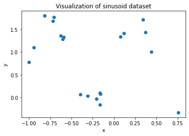
The code snippet below is dedicated to generating the toy dataset in this article, where the value of interest of the data \(y\) is modelled by the sine wave of its feature \(x\) and perturbed by a Gaussian noise \(\mathcal{N}(\mu_{true}=0.8, \sigma^2_{true}=0.02)\). In other words,
and
$$ \begin{equation} \epsilon \sim \mathcal{N}(\mu_{true}=0.8, \sigma^2_{true}=0.02) \end{equation} $$
## Import necessary packages
import numpy as np
import matplotlib.pyplot as plt
import seaborn as sns
from sklearn.metrics import mean_squared_error
np.random.seed(1) # For reproducibility purpose

## Declare the range of x values used for the entire article
x_min = -1
x_max = 1

## Define true parameters for the noise
sigma_true = np.sqrt(0.02)
mu_true = 0.8

def generate_data(n_points, x_min, x_max):
    '''
        This function generates n data points in which their x values are stayed within the interval
        [x_min, x_max), and their y values will be the sine wave of the x values
        and then perturbed by the Gaussian noise N(mu_true, sigma_true^2)

        Parameters
        ----------
        n_points: Number of data points to be generated

        x_min: Minimum x value

        x_max: Maximum x value

        Return
        ------
        data: The (n_points, 2) sinusoid dataset
    '''
    floatinfo = np.finfo(float)
    # floatinfo.eps is the smallest change to make a value greater than 1.0
    x_range = x_max - x_min + floatinfo.eps
    xs = np.random.rand(n_points) * x_range + x_min
    ys = np.sin(2 * np.pi * xs) + (np.random.randn(n_points) * sigma_true + mu_true)
    data = np.concatenate([xs.reshape(-1, 1), ys.reshape(-1, 1)], axis=1)
    return data

## Generate dataset containing 20 data points
dataset = generate_data(20, x_min, x_max)

## Visualize dataset
xs = dataset[:, 0]
ys = dataset[:, 1]
_ = plt.scatter(xs, ys)
plt.xlabel('x')
plt.ylabel('y')
plt.title('Visualization of sinusoid dataset')
plt.show()
2.2 Define linear models
Since the target values of the toy dataset mentioned in the previous section are continuous, the task therefore is a curve-fitting problem. Specifically, to approximate the sine wave \(y = sin(x)\), polynomial regression models with various degrees and a linear combination of Radial Basis Function (RBF) kernels shall be used to examine which types of models provide a good generalizability for both the observed and unobserved data. About polynomial regression models, they are of the form:
Regarding the model containing RBF kernels, it can be expressed as follows:
where,
\(\quad\quad \mu_i\) defines the location in the input space that makes the function return the highest output value, which is 1
\(\quad\quad \sigma_i\) defines how far the input value \(x\) can vary around the mean \(\mu_i\) so that the output of the function is not asymptotically close to 0
def transform_polynomial(xs, degree):
    '''
        Transform the data with single independent variable x into D exponent variables,
        where the largest exponent variable is the original variable power of D.
        For example, suppose x is the original independent variable, if degree=2, then x -> [1 x x^2]

        Parameters
        ----------
        xs: Input vector containing n values of the independent variable x

        degree: Highest degree of the polynomial

        Return
        ------
        new_xs: (n, degree+1) matrix, where degree+1 columns represent the exponents of
                the polynomial in increasing order
    '''
    n_points = len(xs)
    new_xs = np.zeros([n_points, degree+1])
    for i in range(degree+1):
        new_xs[:, i] = xs ** i
    return new_xs

def transform_rbf(xs, mus, sigmas):
    '''
        Transform the data via using RBF kernels. Specifically,
        the single independent variable x will be mapped to d+1 features,
        where the last d features are the outputs d different RBF kernels
        with their mean and shape parameters specified in `mus` and `sigmas` vectors respectively,
        and the first feature is a constant value 1, which is used for bias parameter.

        Parameters
        ----------
        xs: Input vector containing n values of the independent variable x

        mus: Vector of mean parameters for different kernels

        sigmas: Vector of shape parameters for different kernels

        Return
        ------
        new_xs: (n, d+1) matrix
    '''
    n_kernels = len(mus)
    n_points = len(xs)
    new_xs = np.zeros([n_points, n_kernels+1])
    for i in range(n_kernels):
        sigma_sq = sigmas[i] ** 2
        new_xs[:, i+1] = np.exp(-((xs - mus[i]) ** 2) / (2 * sigma_sq))
    new_xs[:, 0] = 1
    return new_xs
3 Posterior Distribution over model parameters \(\mathbf{w}\)
In this section, the main interest is to sampling the model parameters \(\mathbf{w}\) from either the posterior distribution \(p(\mathbf{w}, \beta\) | \(\mathbf{y}, \alpha)\) if the precision parameter of the noise \(\beta\) is unknown, or the posterior distribution \(p(\mathbf{w}\)| \(\mathbf{y}, \beta, \alpha)\) given that \(\beta\) is known, because finding the model parameters that can maximize the posterior distribution is easy once the sampling process is feasible. Therefore, 3 different approaches to sampling from the posterior distribution shall be introduced, where the first approach is directly evaluating the posterior distribution \(p(\mathbf{w}\) | \(\mathbf{y}, \beta, \alpha)\). More importantly, if the posterior distribution is analytically intractable (i.e., it does not have the form of any known mathematical distribution), it is infeasible to sampling the data from the distribution directly. Luckily, with the help of Markov Chain Monte Carlo (MCMC) methods, the data drawn via these methods shall asymptotically follow the intractable distribution. Therefore, two different MCMC methods, which are Metropolis Hasting and Gibbs Sampling, are also introduced in this section to illustrate the sampling process for an intractable posterior distribution.
3.1 Direct Evaluation
According to Bayes’ theorem, the posterior distribution of the model parameters \(\mathbf{w}\) as well as the hyperparameter of the noise \(\beta\) given the data can be defined as follows:
Based on the definition of the posterior distribution of \(\mathbf{w}\) and \(\beta\) in Equation \((1)\), if the precision parameter \(\beta\) is assumed to be known, the posterior distribution of the model parameters \(\mathbf{w}\) now is now simply the posterior distribution of \(\mathbf{w}\) given the data and \(\beta\), which is
where,
\(\quad\quad \boldsymbol{\Phi} = \begin{pmatrix} \boldsymbol{\phi}(\mathbf{x}_1)^T \\ \boldsymbol{\phi}(\mathbf{x}_2)^T \\ \vdots \\ \boldsymbol{\phi}(\mathbf{x}_N)^T \end{pmatrix}\) contains the outputs of the basis functions whose inputs are the features associated with \(N\) data points
\(\quad\quad \mathbf{y} = \begin{pmatrix} y_1 \\ y_2 \\ \vdots \\ y_N\end{pmatrix}\) contains the target values of \(N\) data poitns
Rearranging Equation \((2)\) yields:
Because \(ln(p(\mathbf{w}|\mathbf{y}, \alpha, \beta)) \propto -\frac{1}{2}(\mathbf{w} - \mathbf{m})^T\mathbf{A}(\mathbf{w} - \mathbf{m})\), which has the form of the Gaussian kernel with mean \(\mathbf{m}\) and covariance \(\mathbf{A}^{-1}\). Therefore,
Note that, in practice, we’re usually interested in the predictive distribution of the target values for unseen data but not the posterior distribution over the model parameters given data. Nevertheless, analyzing the posterior distribution over model parameters \(\mathbf{w}\) given data, \(\alpha\), and \(\beta\) is a prerequisite step to evaluate the evidence distribution of the data given \(\alpha\) and \(\beta\), which shall be discussed in Chapter \(\mathbf{5}\). Consequently, the next chapter shall focus on evaluating the predictive distribution of Linear Regression model.
3.2 Metropolis Hasting (MH)
Suppose \(p(x)\) is an intractable distribution that one can only know the form of it up to a constant, for example, \(p(x) \propto x^2 \exp(-x^2 + \sin(x))\). To draw samples from the distribution via Metropolis Hasting algorithm, it can be summarized as follows:
where,
\(\quad\quad q(y|x)\) is a proposal distribution to draw a new sample \(Y\) based on the previous sample \(x\), which is a tractable distribution defined by users. In the sense of Markov Chain, \(q(y|x)\) is referred to the transition probability from state \(x\) to state \(y\)
\(\quad\quad \alpha(x, y) = \min(1, \frac{q(x|y) * p(y)}{q(y|x) * p(x)})\) is the acceptance probability that the sample drawn from the distribution \(q(y|x)\), \(Y=y\), will be accepted as the next sample instead of keeping the previous sample \(x\)
In particular, suppose that the posterior distribution \(p(\mathbf{w}|\mathbf{y}, \beta, \alpha)\) is intractable, and one wishes to sampling from the posterior distribution via Metropolis Hasting algorithm. Define \(\mathbf{W}_t \sim \mathcal{N}(\mathbf{w}_t|\mathbf{w}_{t-1}, \mathbf{C})\) as the proposal distribution, where \(\mathbf{C}\) is designed by users, and \(p(\mathbf{w}|\mathbf{y}, \beta, \alpha)\) as the target distribution to sampling from. Thus, the acceptance probability can be expressed as:
It is worth noted that the posterior distribution \(p(\mathbf{w}|\mathbf{y}, \beta, \alpha)\) is assumed to be intractable and thus it is of the form \(p(\mathbf{w}|\mathbf{y}, \beta, \alpha) \propto p(\mathbf{y}|\mathbf{w}, \beta) * p(\mathbf{w}|\alpha)\). As a result,
3.3 Gibbs Sampling
Similar to MH algorithm, this algorithm is the special case of MH algorithm in which the acceptance rate is always 1, which means that the sample drawn from the proposal distribution is always accepted as a new sample drawn from the target distribution. However, the main difference is that each component of a sample is drawn sequentially from the condition distribution derived from the target distribution, where all other components are fixed. Specifically, suppose that \(\mathbf{X} = \begin{pmatrix} X^{(1)} & X^{(2)} & \cdots & X^{(d)} \end{pmatrix}^T \sim p(\mathbf{x})\) in which the distribution \(p(\mathbf{x})\) is intractable, the procedure to sampling from this distribution via Gibbs Sampling can be described as follows:
Therefore, the most important part to use Gibbs Sampling is to derive the conditional distributions for all components from the target distribution such that these conditional distributions are tractable, which is not always feasible. Returning back to the posterior distribution mentioned in Equation \((1)\), suppose that \(\beta \sim Gamma(a, b)\), where \(a\) and \(b\) are two hyperparameters for the Gamma distribution, the posterior distribution \(p(\mathbf{w}, \beta|\mathbf{y}, \alpha, a, b)\) can be represented as:
To draw samples from this posterior distribution via Gibbs Sampling, we need to derive \(p(\mathbf{w}|\mathbf{y}, \beta, \alpha, a, b)\) and \(p(\beta|\mathbf{y}, \mathbf{w}, \alpha, a, b)\) in order to sequentially sampling \(\mathbf{w}\) and \(\beta\). Note that because the Gamma distribution conjugates to Normal distribution, the conditional distribution \(p(\beta|\mathbf{w}, \mathbf{y}, \alpha, a, b)\) therefore is another Gamma distribution. To be clear,
Now, it remains to derive \(p(w_i|\mathbf{y}, \{w_j\}_{j \neq i}, \beta, \alpha, a, b)\) in order to use Gibbs Sampling, where \(\mathbf{w} = \begin{pmatrix}w_0 & \cdots & w_i & \cdots & w_{M-1}\end{pmatrix}^T\). Expanding \(p(w_i|\mathbf{y}, \{w_j\}_{j \neq i}, \beta, \alpha, a, b)\) and completing the square gives:
3.4 Define the procedure to sampling model parameters \(\mathbf{w}\) from the posterior distribution
3.4.1 Direct evaluation
def sampling_model_posterior(X, y, beta, alpha):
    '''
        This function sampling the model parameters of a linear model from the posterior
        distribution as described in Equation (4)

        Parameters
        ----------
        X: (n_points, n_features) matrix in which each row is the feature vector of a data point

        y: n_points-dimensional vector in which each row is the target value of a data point

        beta: precision parameter associated with the noise of the target values,
                which is mentioned in Chapter 2 - Model Assumption

        alpha: precision parameter associated with the prior of model parameters,
                which is mentioned in Chapter 2 - Model Assumption

        Return
        ------
        mean_posterior, cov_posterior, w_posterior: mean of the posterior distribution,
        covariance matrix of the posterior distribution,
        and the parameters sampled from the posterior distribution in Equation (4)
    '''
    n_features = X.shape[1]
    precision_posterior = (beta*X.T @ X) + (alpha * np.eye(n_features)) # A
    # Solve a system of equations A*X = I to find X,
    # where X in this case is actually the inverse of A
    cov_posterior = np.linalg.solve(precision_posterior, np.eye(precision_posterior.shape[0])) # A^-1
    mean_posterior = (beta * cov_posterior) @ (X.T @ y) #  m
    w_posterior = np.random.multivariate_normal(mean_posterior, cov_posterior)
    return mean_posterior, cov_posterior, w_posterior
3.4.2 Metropolis Hasting
def MH_sampling_model_posterior(X, y, beta, alpha, n_samples=10000, burnin_size=500):
    '''
        This function sampling the model parameters of a linear model
        from the posterior distribution p(w|y, beta, alpha) via Metropolis Hasting algorithm

        Parameters
        ----------
        X: (n_points, n_features) matrix in which each row is the feature vector of a data point

        y: n_points-dimensional vector in which each row is the target value of a data point

        beta: precision parameter associated with the noise of the target values,
                which is mentioned in Chapter 2 - Model Assumption

        alpha: precision parameter associated with the prior of model parameters,
                which is mentioned in Chapter 2 - Model Assumption

        n_samples: Number of samples to be drawn from the posterior distribution

        burnin_size: Number of first samples to be discarded during the sampling process

        Return
        ------
        W, pdfs: (n_samples, n_features) matrix contains the samples drawn
                from the posterior distribution and a n_samples-dimensional vector
                contains the unnormalized densities of those samples respectively
    '''
    n_features = X.shape[1]
    # Unnormalized expression for the posterior distribution of w|y, beta, alpha
    posterior_pdf = lambda w: np.exp(-(beta / 2) * (np.linalg.norm(y - (X @ w)) ** 2)) * \
                                np.exp(-(alpha / 2) * (w.T @ w))
    W = np.zeros([n_samples, n_features])
    pdfs = np.zeros(n_samples)
    w_accepted = np.random.rand(n_features)
    n_accepted = 0
    # covariance matrix for the proposal distribution,
    # which can be tuned to have more accepted samples
    C = np.eye(n_features)
    C[C != 0] = 0.05
    for t in range(n_samples + burnin_size):
        w_proposal = np.random.multivariate_normal(mean=w_accepted, cov=C)
        acceptance_prob = min(1, posterior_pdf(w_proposal) / posterior_pdf(w_accepted))
        # If the proposal weights are more promising, accept it
        if np.random.rand() <= acceptance_prob:
            w_accepted = w_proposal
            n_accepted += 1
        # Store the sampled values
        W[t-burnin_size, :] = w_accepted.copy()
        pdfs[t-burnin_size] = posterior_pdf(w_accepted)
    print('Number of accepted samples via MH algorithm: {}'.format(n_accepted))
    return W, pdfs
3.4.3 Gibbs Sampling
def Gibbs_sampling_model_posterior(X, y, alpha, beta=None, n_samples=2000, burnin_size=500):
    '''
        This function sampling the model parameters of a linear model
        from the posterior distribution p(w, beta|y, alpha) via Gibbs Sampling algorithm

        Parameters
        ----------
        X: (n_points, n_features) matrix in which each row is the feature vector of a data point

        y: n_points-dimensional vector in which each row is the target value of a data point

        alpha: precision parameter associated with the prior of model parameters,
                which is mentioned in Chapter 2 - Model Assumption

        beta: precision parameter associated with the noise of the target values,
                which is mentioned in Chapter 2 - Model Assumption,
                if beta is given, the algorithm will use it to sampling another not given parameters,
                otherwise, this parameter will also be sampled along with other parameters

        n_samples: Number of samples to be drawn from the posterior distribution

        burnin_size: Number of first samples to be discarded during the sampling process

        Return
        ------
        betas, W, pdfs: n_samples-dim vector contains the precision values of the data noise and
                (n_samples, n_features) matrix contains the model parameters and
                n_samples-dim vector contains the unnormalized densities of those samples
                drawn from the posterior distribution repsectively
    '''
    n_features = X.shape[1]
    n_training_samples = X.shape[0]
    # Unnormalized expression for the posterior distribution of w, beta|y, alpha, a=1, b=1, which is
    # Normal(y|w^Tx, beta^-1) * Normal(alpha|0, alpha^-1) * Gamma(beta|a=1, b=1)
    posterior_pdf = lambda w, beta: np.exp(-(beta / 2) * (np.linalg.norm(y - (X @ w)) ** 2)) * \
                                np.exp(-(alpha / 2) * (w.T @ w)) * \
                                np.exp(-beta)
    W = np.zeros([n_samples, n_features])
    betas = np.zeros(n_samples)
    pdfs = np.zeros(n_samples)
    w = np.random.rand(n_features)
    is_beta_given = beta is not None
    if not is_beta_given:
        beta = np.random.uniform(1, 10)
    for t in range(n_samples + burnin_size):
        ## Sampling beta
        if not is_beta_given:
            # First parameter for the conditional Gamma distribution, where a is set to 1
            a_ = 1 + (n_training_samples / 2)
            # Second parameter for the conditional Gamma distribution, where b is set to 1
            b_ = 1 + (1 / 2) * (np.linalg.norm(y - (X @ w)) ** 2)
            beta = np.random.gamma(shape=a_, scale=b_)
        ## Sampling model weights w
        for feature_idx in range(n_features):
            s = beta * np.sum(X[:, feature_idx] ** 2) + alpha
            s_inv = 1 / s
            k = s_inv * beta * np.sum(
                X[:, feature_idx] * (y - (X @ w) + (X[:, feature_idx] * w[feature_idx]))
            )
            w[feature_idx] = np.random.normal(loc=k, scale=s_inv ** (0.5))
        ## Store the sampled values
        W[t-burnin_size, :] = w.copy()
        betas[t-burnin_size] = beta
        pdfs[t-burnin_size] = posterior_pdf(w, beta)
    return betas, W, pdfs
3.5 Create datasets for polynomial models and RBF-kernel models
## Compose datasets for polynomial models
min_deg = 1 # Minimum degree of polynomial
max_deg = 10 # Maximum degree of polynomial
datasets_polynomial = [
    np.concatenate([transform_polynomial(xs, deg), ys.reshape(-1, 1)], axis=1)
    for deg in range(min_deg, max_deg + 1)
]

## Compose datasets for RBF-kernel models,
## where the means of kernels shall be determined by K-Means clustering algorithm
## to ensure that all the points having similar cluster should be well expressed
## by a common kernel with mean = their centroid
## About the shape parameters, they can be optimized via LOOCV,
## but here I manually checked it and found that shape parameter = 0.3 can approximate
## the data reasonably well.
## Therefore, shape parameter is assumed to be 0.3 for all rbf kernels
from sklearn.cluster import KMeans
min_n_kernels = 1 # Minimum number of RBF kernels
max_n_kernels = 10 # Maximum number of RBF kernels
params_rbf = {} # Store the specified kernel parameters for different RBF-kernel models
for n_kernels in range(min_n_kernels, max_n_kernels+1):
    kmeans = KMeans(n_clusters=n_kernels, random_state=0).fit(xs.reshape(-1, 1))
    # Calculate the mean and the shape values for each kernel
    params_rbf[n_kernels] = {'mean': [], 'shape': []}
    for label in np.unique(kmeans.labels_):
        mean = np.mean(xs[kmeans.labels_ == label])
        std = 0.3
        params_rbf[n_kernels]['mean'].append(mean)
        params_rbf[n_kernels]['shape'].append(std)

datasets_rbf = [
    np.concatenate([transform_rbf(
        xs,
        params_rbf[n_kernels]['mean'],
        params_rbf[n_kernels]['shape']
    ), ys.reshape(-1, 1)], axis=1) for n_kernels in range(min_n_kernels, max_n_kernels+1)
]
3.6 Visualize samples drawn by 3 different approaches
Since it is hard to visualize a multi-dimensional parameter space, I will opt for plotting the model parameter space in 2D plane, where the model is a linear model with 2 RBF kernels and the bias term is kept fixed at the value evaluated from the true posterior distribution in Equation \((4)\).
def w_true_posterior_pdf(w, mean, cov, w_bias=None):
    '''
        This function computes the pdf of the posterior distribution over model parameters w,
        which is p(w|y, beta, alpha) described in Equation (4)

        Parameters
        ----------
        w: Input model parameters, which can be a 2D meshgrid containing sets of parameters
            or a single vector of n_features dimensions

        mean: mean of the posterior distribution

        cov: covariance matrix of the posterior distribution

        w_bias: posterior mean for the bias parameter, if set to not None,
                w_bias will be concatenated with w to feed into the posterior pdf

        Return
        ------
        result: pdf for w evaluated by p(w|y, beta, alpha), which has the same shape of w
    '''
    n_features = len(mean)
    pdf = lambda w: ((2 * np.pi) ** (-n_features / 2)) * (np.linalg.det(cov) ** (-0.5)) * \
                    np.exp(-0.5 * (w - mean).T @ np.linalg.inv(cov) @ (w - mean))

    result = 0
    if type(w) == list: # w is a meshgrid
        w1s = w[0]
        w2s = w[1]
        result = np.zeros(w[0].shape)
        for idx, _ in np.ndenumerate(w1s):
            weights = np.array([w_bias, w1s[idx], w2s[idx]]) if w_bias \
                    else np.array([w1s[idx], w2s[idx]])
            result[idx] = pdf(weights)
    else: # w is just a vector of parameters
        result = pdf(w)
    return result
## Generate data to sketch contour plot for the true posterior distribution
## + samples generated via MH and Gibbs algorithms
# Get the true posterior mean and the posterior covariance evaluated by Equation (4)
w_posterior_mean, w_posterior_cov, _ = sampling_model_posterior(
    datasets_rbf[1][:, :-1], datasets_rbf[1][:, -1], beta=1/(sigma_true ** 2), alpha=1/0.02
)
bias_posterior_mean = w_posterior_mean[0]
# Create grid of model parameters w1 and w2 and evaluate their density,
# where w = (w0, w1, w2)^T and w0 is the bias term
w1s = np.linspace(w_posterior_mean[1] - 5 * (w_posterior_cov[1, 1] ** (0.5)),
                w_posterior_mean[1] + 5 * (w_posterior_cov[1, 1] ** (0.5)),
                1000)
w2s = np.linspace(w_posterior_mean[2] - 5 * (w_posterior_cov[2, 2] ** (0.5)),
                w_posterior_mean[2] + 5 * (w_posterior_cov[2, 2] ** (0.5)),
                1000)
W = np.meshgrid(w1s, w2s)

posterior_pdfs = w_true_posterior_pdf(W, w_posterior_mean, w_posterior_cov, bias_posterior_mean)

# Sampling model parameters via MH algorithm through
# the intractable form of the posterior distribution
w_samples_MH, pdfs_MH = MH_sampling_model_posterior(
    datasets_rbf[1][:, :-1], datasets_rbf[1][:, -1], beta=1/(sigma_true ** 2), alpha=1/0.02
)
# Sampling model parameters via Gibbs algorithm through
# the intractable form of the posterior distribution
beta_samples_Gibbs, w_samples_Gibbs, pdfs_Gibbs = Gibbs_sampling_model_posterior(
    X=datasets_rbf[1][:, :-1], y=datasets_rbf[1][:, -1], alpha=1/0.02
)
Number of accepted samples via MH algorithm: 412
plt.figure(figsize=(8, 8))
plt.contour(w1s, w2s, posterior_pdfs, cmap='RdGy')
plt.scatter(w_posterior_mean[1], w_posterior_mean[2], c='red',
            label='True Posterior Mode'
)
plt.scatter(w_samples_Gibbs[:, 1], w_samples_Gibbs[:, 2], s=1, c='blue',
            label='Samples via Gibbs algorithm'
)
plt.scatter(w_samples_MH[:, 1], w_samples_MH[:, 2], c='green', s=1,
            label='Samples via MH algorithm'
)
plt.xlabel('w1')
plt.ylabel('w2')
plt.legend()
plt.title(
    r'Contour plot of the true posterior distribution $p(\mathbf{w}|\mathbf{y}, \beta, \alpha)$' +
          '\n and the samples generated via MH and Gibbs algorithms'
)
plt.show()
print('True Posterior Mode: {}'.format(w_posterior_mean[1:]))
print('Posterior Mode via MH: {}'.format(w_samples_MH[np.argmax(pdfs_MH)][1:]))
print('Posterior Mode via Gibbs: {}'.format(w_samples_Gibbs[np.argmax(pdfs_Gibbs)][1:]))
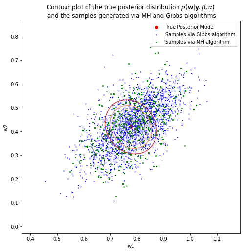
True Posterior Mode: [0.77630428 0.4187777 ]
Posterior Mode via MH: [0.79404474 0.4412848 ]
Posterior Mode via Gibbs: [0.59198952 0.35997657]
Clearly, the number of accepted samples in MH algorithm is much less than the desired number of samples that we wish to sampling from, which is only 412 over 10000 samples, and this inefficiency happens due to the design of the covariance matrix for the proposal distribution. Therefore, the obvious ways to increase the acceptance rate in MH algorithm are to tune the covariance matrix for the proposal distribution or to try another type of distributions. About the Gibbs Sampling algorithm, even though more samples can be generated compared to using MH algorithm, the posterior mode however estimated by Gibbs Sampling is far removed from the true posterior mode. The reason for this is because I use Gibbs Sampling to estimate both the model parameters \(\mathbf{w}\) as well as the precision of the noise \(\beta\), while the true value of \(\beta\) is given to MH algorithm to estimate the posterior mode, and thus the posterior mode of MH algorithm is close to the true posterior mode.
To overcome this limitation when using Gibbs Sampling, let’s visualize the distribution of \(\beta\) and pick the most evident value and keep it fixed during the sampling process:
## Visualize the distribution of the beta parameter sampled via Gibbs Sampling
kde = sns.kdeplot(beta_samples_Gibbs)
plt.xlabel(r'$\beta$')
plt.title('KDE plot for beta values sampled from Gibbs Sampling')
plt.show()
x, y = kde.get_lines()[0].get_data()
print('Mode of beta: {}'.format(x[np.argmax(y)]))
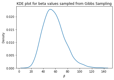
Mode of beta: 51.90096574793529
Visually speaking, the mode for \(\beta\) is close to the true value, which is 50. In this case, the estimated mode of \(\beta\) is 51.9. Now, let’s fix \(\beta = 51.9\) and use Gibbs Sampling to draw model parameters \(\mathbf{w}\) from the posterior distribution and check whether the posterior mode is going to be close to the true posterior mode.
## Generate samples via Gibbs Sampling while keeping beta=51.9
beta_samples_Gibbs, w_samples_Gibbs, pdfs_Gibbs = Gibbs_sampling_model_posterior(
    X=datasets_rbf[1][:, :-1], y=datasets_rbf[1][:, -1], alpha=1/0.02, beta=51.9
)
## Visualize it
plt.figure(figsize=(8, 8))
plt.contour(w1s, w2s, posterior_pdfs, cmap='RdGy')
plt.scatter(w_posterior_mean[1], w_posterior_mean[2], c='red', label='True Posterior Mode')
plt.scatter(w_samples_Gibbs[:, 1], w_samples_Gibbs[:, 2], s=1, c='blue', label='Samples via Gibbs algorithm')
plt.xlabel('w1')
plt.ylabel('w2')
plt.legend()
plt.title(
    r'Contour plot of the true posterior distribution $p(\mathbf{w}|\mathbf{y}, \beta, \alpha)$' +
          '\n and the samples generated via Gibbs Sampling'
)
plt.show()
print('True Posterior Mode: {}'.format(w_posterior_mean[1:]))
print('Posterior Mode via Gibbs: {}'.format(w_samples_Gibbs[np.argmax(pdfs_Gibbs)][1:]))
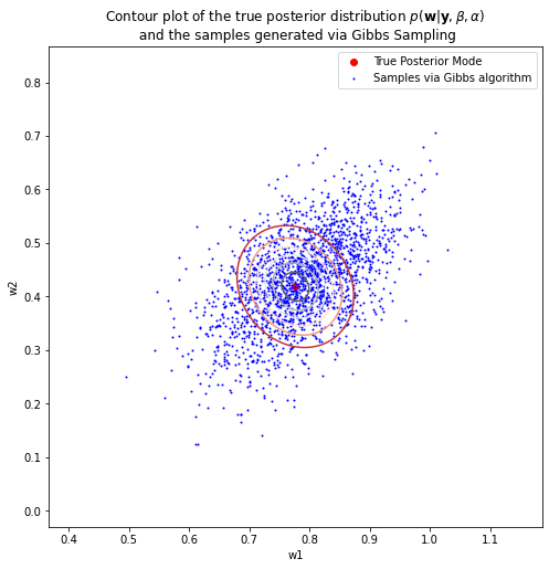
True Posterior Mode: [0.77630428 0.4187777 ]
Posterior Mode via Gibbs: [0.78784972 0.42463967]
Quantitatively speaking, the posterior mode approximated by Gibbs Sampling is now highly similar to the true posterior mode, which addresses the problem that I have previously demonstrated when using Gibbs Sampling.
3.7 Sampling model parameters \(\mathbf{w}\) from the posterior distribution and visualize how well the sampled model parameters fit the data
def make_prediction(xs, w, model_info):
    '''
        This function predicts the target values for all values in xs of the independent variable
        based on the given model parameters w and the type of the model (e.g., polynomial or rbf)

        Parameters
        ----------
        xs: Input vector containing values of the independent variable x

        w: Model parameters

        model_info: A dictionary contains model type and model hyperparameters

        Return
        ------
        ys_hat: Predicted values for all values in xs
    '''
    n_features = w.shape[0] - 1 # Number of basis functions excluding the bias
    if model_info['type'] == 'polynomial':
        xs_transformed = transform_polynomial(xs, n_features)
    elif model_info['type'] == 'rbf':
        mus = model_info['mean']
        sigmas = model_info['shape']
        xs_transformed = transform_rbf(xs, mus, sigmas)
    ys_hat = xs_transformed @ w
    return ys_hat
3.7.1 Visualize predictions of polynomial models inferred from the posterior distribution
x_min_ = np.min(xs) - 0.1
x_max_ = np.max(xs) + 0.1
all_xs = np.linspace(x_min_, x_max_, 1000)

fig, axs = plt.subplots(nrows=2, ncols=2, sharex=True, sharey=True, figsize=(10, 10))

# Sketch 1-degree polynomial model on the top left plot
axs[0, 0].scatter(xs, ys)
for i in range(5):
    # Sampling model parameters w
    w = sampling_model_posterior(datasets_polynomial[0][:, :-1], datasets_polynomial[0][:, -1], 1/0.05, 1/0.02)[2]
    # Plot the model prediction vs data
    axs[0, 0].plot(all_xs, make_prediction(all_xs, w, {'type':'polynomial'}), c='red')
axs[0, 0].set_title('1-degree polynomial regression')
# Sketch 3-degree polynomial model on the top right plot
axs[0, 1].scatter(xs, ys)
for i in range(5):
    # Sampling model parameters w
    w = sampling_model_posterior(datasets_polynomial[2][:, :-1], datasets_polynomial[2][:, -1], 1/0.05, 1/0.02)[2]
    # Plot the model prediction vs data
    axs[0, 1].plot(all_xs, make_prediction(all_xs, w, {'type':'polynomial'}), c='green')
axs[0, 1].set_title('3-degree polynomial regression')
# Sketch 5-degree polynomial model on the bottom left plot
axs[1, 0].scatter(xs, ys)
for i in range(5):
    # Sampling model parameters w
    w = sampling_model_posterior(datasets_polynomial[4][:, :-1], datasets_polynomial[4][:, -1], 1/0.05, 1/0.02)[2]
    # Plot the model prediction vs data
    axs[1, 0].plot(all_xs, make_prediction(all_xs, w, {'type':'polynomial'}), c='blue')
axs[1, 0].set_title('5-degree polynomial regression')
# Sketch 8-degree polynomial model on the bottom right plot
axs[1, 1].scatter(xs, ys)
for i in range(5):
    # Sampling model parameters w
    w = sampling_model_posterior(datasets_polynomial[7][:, :-1], datasets_polynomial[7][:, -1], 1/0.05, 1/0.02)[2]
    # Plot the model prediction vs data
    axs[1, 1].plot(all_xs, make_prediction(all_xs, w, {'type':'polynomial'}), c='orange')
axs[1, 1].set_title('8-degree polynomial regression')
plt.show()
3.7.2 Visualize predictions of RBF-kernel models inferred from the posterior distribution
x_min_ = np.min(xs) - 0.1
x_max_ = np.max(xs) + 0.1
all_xs = np.linspace(x_min_, x_max_, 1000)

fig, axs = plt.subplots(nrows=2, ncols=2, sharex=True, sharey=True, figsize=(10, 10))

# Sketch 1-rbf-kernel model on the top left plot
axs[0, 0].scatter(xs, ys)
for i in range(5):
    # Sampling model parameters w
    w = sampling_model_posterior(datasets_rbf[0][:, :-1], datasets_rbf[0][:, -1], 1/0.05, 1/0.02)[2]
    # Plot the model prediction vs data
    axs[0, 0].plot(
        all_xs, make_prediction(all_xs, w, {'type':'rbf', 'mean': params_rbf[1]['mean'], 'shape': params_rbf[1]['shape']}),
        c='red'
    )
axs[0, 0].set_title('Linear regression with 1 RBF kernels')
# Sketch 3-degree polynomial model on the top right plot
axs[0, 1].scatter(xs, ys)
for i in range(5):
    # Sampling model parameters w
    w = sampling_model_posterior(datasets_rbf[2][:, :-1], datasets_rbf[2][:, -1], 1/0.05, 1/0.02)[2]
    # Plot the model prediction vs data
    axs[0, 1].plot(
        all_xs, make_prediction(all_xs, w, {'type':'rbf', 'mean': params_rbf[3]['mean'], 'shape': params_rbf[3]['shape']}),
        c='green'
    )
axs[0, 1].set_title('Linear regression with 3 RBF kernels')
# Sketch 5-rbf-kernel model on the bottom left plot
axs[1, 0].scatter(xs, ys)
for i in range(5):
    # Sampling model parameters w
    w = sampling_model_posterior(datasets_rbf[4][:, :-1], datasets_rbf[4][:, -1], 1/0.05, 1/0.02)[2]
    # Plot the model prediction vs data
    axs[1, 0].plot(
        all_xs, make_prediction(all_xs, w, {'type':'rbf', 'mean': params_rbf[5]['mean'], 'shape': params_rbf[5]['shape']}),
        c='blue'
    )
axs[1, 0].set_title('Linear regression with 5 RBF kernels')
# Sketch 9-rbf-kernel model on the bottom right plot
axs[1, 1].scatter(xs, ys)
for i in range(5):
    # Sampling model parameters w
    w = sampling_model_posterior(datasets_rbf[8][:, :-1], datasets_rbf[8][:, -1], 1/0.05, 1/0.02)[2]
    # Plot the model prediction vs data
    axs[1, 1].plot(
        all_xs, make_prediction(all_xs, w, {'type':'rbf', 'mean': params_rbf[9]['mean'], 'shape': params_rbf[9]['shape']}),
        c='orange'
    )
axs[1, 1].set_title('Linear regression with 9 RBF kernels')
plt.show()
4 Predictive Distribution
Suppose \((\mathbf{x}^*, y^*)\) is a new data point in which \(\mathbf{x}^*\) is given and \(y^*\) is unknown, the task now is to infer the predictive distribution of \(y^*\) given the available dataset \(\mathcal{D} = \{(\mathbf{x}_1, y_1), ..., (\mathbf{x}_N, y_N)\}\) and other hyperparameters associated with the model and the data, which are \(\beta\) and \(\alpha\). In other words, we wish to find \(p(y^*|\mathbf{y}, \beta, \alpha)\), which is the compact representation of the predictive distribution of unseen data given available data. Now, expanding \(p(y^*|\mathbf{y}, \beta, \alpha)\) yields:
Define:
By completing the square with resepct to \(\mathbf{w}\) with the help of \((5)\) and \((6) \Rightarrow\)
Define:
Using Woodbury matrix inversion lemma on \(\Lambda\) and \(\mathbf{B}\) yields:
From \((8)\) and \((9) \Rightarrow\)
Substitute \((8)\) and \((10)\) into \((7)\):
It is obvious that the predictive mean of \(y^*\) about an unseen data point is essentially the linear combination of the basis functions, where the inputs are the given features of that data point, and those functions are weighted by the posterior mean of model parameters \(\mathbf{m}\). To provide more insights about the predictive mean of \(y^*\), expanding \(\mu\) gives:
Based on Equation \((12)\), the predictive mean of \(y^*\) can be interpreted as the weighted average of the target values \(y_i\) with regard to the observed data points, where the weight associated with a data point \(i\) is evaluated by applying the linear smoother of the form \(k(\mathbf{a}, \mathbf{b}) = \boldsymbol\phi(\mathbf{a})^T\mathbf{A}^{-1}\boldsymbol\phi(\mathbf{b})\) on \(\mathbf{x}_i\) and \(\mathbf{x}^*\)
4.1 Define procedure for sampling models parameters from the predictive distribution
def sampling_model_predictive(x, X, y, beta, alpha):
    '''
        This function sampling the model parameters of a linear model from the predictive distribution
        as described in Equation (11)

        Parameters
        ----------
        x: A feature vector of the unseen data point

        X: (n_points, n_features) matrix in which each row is the feature vector of a training data point

        y: n_points-dimensional vector in which each row is the target value of a data point

        beta: precision parameter associated with the noise of the target values,
                which is mentioned in Chapter 2 - Model Assumption

        alpha: precision parameter associated with the prior of model parameters,
                which is mentioned in Chapter 2 - Model Assumption

        Return
        ------
        mean_predictive, std_predictive, w_predictive: mean of the predictive distribution,
            standard deviation of the predictive distribution,
            and model parameters sampled from the predictive distribution in Equation (11)
            to predict the target value of the unseen data point
    '''
    n_features = X.shape[1]
    mean_posterior, cov_posterior, _ = sampling_model_posterior(X, y, beta, alpha)
    var_predictive = (1 / beta) + ((x.T @ cov_posterior) @ x) # Equation (9)
    std_predictive = np.sqrt(var_predictive)
    mean_predictive = x.T @ mean_posterior # Equation (10)
    w_predictive = np.random.normal(loc=mean_predictive, scale=std_predictive)
    return mean_predictive, std_predictive, w_predictive
4.2 Visualize predictions and point-wise confidence intervals of 3-degree polynomial model inferred from the predictive distribution
X_unseen = transform_polynomial(all_xs, 3)
y_pred = np.zeros(X_unseen.shape[0]) # Store the predicted y values of unseen data
y_pred_lb = np.zeros(X_unseen.shape[0]) # Store the lower-bound CI of the predicted y values of unseen data
y_pred_ub = np.zeros(X_unseen.shape[0]) # Store the upper-bound CI of the predicted y values of unseen data
for i, x in enumerate(X_unseen):
    y_pred[i], std, _ = sampling_model_predictive(
        x, datasets_polynomial[2][:, :-1], datasets_polynomial[2][:, -1], 1/0.05, 1/0.2
    )
    y_pred_lb[i] = y_pred[i] - 1.96*std # 95% CI
    y_pred_ub[i] = y_pred[i] + 1.96*std # 95% CI

plt.figure(figsize=(8, 5))
plt.scatter(xs, ys)
plt.plot(all_xs, y_pred, color='red')
plt.fill_between(all_xs, y_pred_lb, y_pred_ub, color='b', alpha=.1)
plt.title('Predictive polynomial model with 3 degree')
plt.xlabel('x')
plt.ylabel('y')
plt.show()
4.3 Visualize predictions and point-wise confidence intervals of 9-RBF-kernel model inferred from the predictive distribution
X_unseen = transform_rbf(all_xs, params_rbf[9]['mean'], params_rbf[9]['shape'])
y_pred = np.zeros(X_unseen.shape[0]) # Store the predicted y values of unseen data
y_pred_lb = np.zeros(X_unseen.shape[0]) # Store the lower-bound CI of the predicted y values of unseen data
y_pred_ub = np.zeros(X_unseen.shape[0]) # Store the upper-bound CI of the predicted y values of unseen data
for i, x in enumerate(X_unseen):
    y_pred[i], std, _ = sampling_model_predictive(x, datasets_rbf[8][:, :-1], datasets_rbf[8][:, -1], 1/0.05, 1/0.2)
    y_pred_lb[i] = y_pred[i] - 1.96*std # 95% CI
    y_pred_ub[i] = y_pred[i] + 1.96*std # 95% CI

plt.figure(figsize=(8, 5))
plt.scatter(xs, ys)
plt.plot(all_xs, y_pred, color='red')
plt.fill_between(all_xs, y_pred_lb, y_pred_ub, color='b', alpha=.1)
plt.title('Predictive RBF-kernel model with 9 basis functions')
plt.xlabel('x')
plt.ylabel('y')
plt.show()
By looking at the predicted results from polynomial models and RBF-kernel models, it is evident that RBF-kernel models fit the data better than polynomial models, and this happens due to RBF functions provide higher complexity in explaining non-linear relationship between variables. About the prediction interval, all the data points are well-captured within the interval suggested by the RBF-kernel model. Whereas, the polynomial model has failed to capture the variability of the target values associated with multiple explanatory values, which therefore make the prediction interval of the model leave many data points outside the bound.
Last but not least, it is worth reminding that the hyperparameters \(\beta\) and \(\alpha\) mentioned in \(\text{Chapter } \mathbf{2}\) are chosen arbitrarily for the implementation of \(\text{ Chapters } \mathbf{3} \space\&\space \mathbf{4}\), which is just to illustrate how the model parameters are inferred from the posterior distribution \(p(\mathbf{w}|\mathbf{y}, \beta, \alpha)\) or the predictive distribution \(p(y^*|\mathbf{y}, \beta, \alpha)\). Hence, it is too soon to conclude that the models with RBF kernels fit the data better than the polynomial models. As a result, the next chapter shall focus on optimizing these two hyperparameters then use the optimized hyperparameters to infer the model parameters so as to rigorously judge which model works best among the proposed models.
5 Evidence Distribution
In Bayesian inference, the term “evidence” is referred to the marginal likelihood distribution of the data, which is essentially the distribution of the observed data marginalized over the model parameters, which is \(p(\mathbf{y}|\beta, \alpha)\) - the denominator of the posterior distribution over the model parameters \(p(\mathbf{w}|\mathbf{y}, \beta, \alpha)\). Integrating \(p(\mathbf{y}|\beta, \alpha)\) over \(\mathbf{w}\) yields:
One may ask why bother mentioning the evidence distribution and how is it related to optimizing \(\beta\) and \(\alpha\), it turns out that choosing the values of \(\beta\) and \(\alpha\) to maximize the evidence distribution is an approximation approach to find the most sensible values of \(\beta\) and \(\alpha\) for maximizing the predictive distribution. To be specific, the next section shall clarify the reason behind maximizing the evidence function with respect to \(\beta\) and \(\alpha\) can lead to maximizing the predictive distribution, which is so called evidence approximation.
5.1 Evidence approximation
In general, to find out the most reasonable target value \(y^*\) for an unseen data point given its observable features \(\mathbf{x}^*\) and other observed data points \((\mathbf{X}, \mathbf{y})\), it is equivalent to finding the predictive distribution \(p(y^*|\mathbf{X}, \mathbf{y}, \mathbf{x}^*)\), which is \(p(y^*|\mathbf{y})\) in short. In this article, because the target variable \(y\) is governed by the linear model with a set of parameters \(\mathbf{w}\), \(\beta\), and \(\alpha\) described in \(\text{Chapter } \mathbf{2}\), the predictive distribution can be thus expressed as follows:
Assuming that the posterior distribution of \(p(\beta, \alpha|\mathbf{y})\) is sharply peaked at \((\hat{\beta}, \hat{\alpha})\), i.e. the density of \(p(\beta, \alpha|\mathbf{y})\) is almost zero everywhere except for the density at \((\hat{\beta}, \hat{\alpha})\), the predictive distribution in Equation \((14)\) can therefore be approximated via:
Based on the assumption given above, it remains to find \(\hat{\beta}\) and \(\hat{\alpha}\) then substitute in Equation \((15)\) in order to approximate the predictive distribution in Equation \((14)\), which is analogous to finding the posterior mode of the distribution \(p(\beta, \alpha|\mathbf{y})\). As a result, this whole process is called evidence approximation. Next, to obtain \(\hat{\beta}\) and \(\hat{\alpha}\), applying Bayes’ theorem on \(p(\beta, \alpha|\mathbf{y})\) gives:
If the prior of \(\beta\) and \(\alpha\) (i.e., \(p(\beta, \alpha)\)) is flat, maximizing the posterior distribution over \(\beta\) and \(\alpha\), \(p(\beta, \alpha|\mathbf{y})\), is equivalent to maximizing the marginal likelihood function of the given data \(\mathbf{y}- p(\mathbf{y}|\beta, \alpha)\), which is the evident distribution in Equation \((13)\). To summarize, the most sensible values of \(\beta\) and \(\alpha\) can be evaluated via maximizing the evidence distribution (i.e., Equation \((13)\)) or the log of the evidence distribution.
5.2 Optimize \(\beta\) and \(\alpha\) via maximizing the log of the evidence distribution
In this section, two approaches shall be demonstrated to optimize \(\beta\) and \(\alpha\). The first one is simply by setting the derivative of the log evidence function by 0 and solve for the parameters of interest to find the optimal values for them. The second approach is by making use of EM algorithm to iteratively obtain the optimal values of \(\beta\) and \(\alpha\).
5.2.1 Derivative approach
Before discussing the method to optimize \(\beta\) and \(\alpha\), consider \(\lambda_i\) and \(\mathbf{u}_i\) are the \(i^{th}\) eigenvalue and the eigenvector of \(\beta\boldsymbol{\Phi}^T\boldsymbol{\Phi}\) respectively, where \(1 \leq i \leq M\). Therefore,
Based on that, the eigen decomposition of \(\alpha\mathbf{I} + \beta\boldsymbol{\Phi}^T\boldsymbol{\Phi}\) can be viewed as:
Note that the determinant of a \(n \times n\) matrix \(\mathbf{M}\) is the product of its eigenvalues. By using the result in Equation \((17)\), \(|\mathbf{A}|\) thereby can be rewritten as:
Taking the logarithm of the evidence distribution and substitute \(|\mathbf{A}|\) by the right hand side of Equation \((18)\) gives:
Setting the derivative of Equation \((19)\) with respect to \(\alpha\) to 0 then solving for \(\alpha\) yields:
Note that this is an implicit solution to compute \(\alpha\) since both \(\gamma\) and \(\mathbf{m} = \beta\mathbf{A}^{-1}\boldsymbol\Phi^T\mathbf{y}\) also depend on \(\alpha\). Thus, to obtain the desirable value of \(\alpha\), one can use Equation \((20)\) as an iterative procedure to compute \(\alpha\) by first setting \(\alpha\) to some initial value to compute \(\mathbf{m}\) and \(\gamma\) in order to estimate \(\alpha\) until convergence. Similarly, \(\beta\) can be optimized via setting the derivative of Equation \((19)\) with respect to \(\beta\) to solve for \(\beta\), which is given as follows:
where, \(\frac{d\lambda_i}{d\beta} = \frac{\lambda_i}{\beta}\) based on the fact that \(\beta\boldsymbol{\Phi}^T\boldsymbol{\Phi} \mathbf{u}_i = \lambda_i \mathbf{u}_i \Leftrightarrow c*\beta\mathbf{u}_i = \lambda_i\mathbf{u}_i\) in which \(c\) is a constant; hence, \(c*\beta = \lambda_i \Leftrightarrow \frac{d\lambda_i}{d\beta} = c = \frac{\lambda_i}{\beta}\)
Observe that Equation \((21)\) is also an implicit solution for obtaining \(\beta\) and thus the optimal value for \(\beta\) can be computed via an iterative approach similar to the update procedure of \(\alpha\). In general, \(\alpha\) and \(\beta\) can be iteratively updated together by first initializing \(\beta\) and \(\alpha\) to compute \(\mathbf{m}\) and \(\gamma\) then using Equations \((20)\) & \((21)\) to recompute \(\beta\) and \(\alpha\) and repeating the process until convergence. Interestingly, the denominator of Bayesian solution to update \(\beta\) is \(N-\gamma\) instead of \(N\) described in Maximum Likelihood Estimation (MLE) solution, which means that the Bayesian solution also takes away some degree of freedom in order to produce an unbiased estimation of the noise variance \(\frac{1}{\beta}\), since the MLE solution for \(\frac{1}{\beta}\) is indeed a biased estimation. What is more, the term \(\gamma\) has an elegant interpretation about the model parameters. That is, it indicates the number of effective parameters in the model (i.e., the parameters significantly differ from 0), and so \(N-\gamma\) determines the total degrees of freedom excluding some degrees of freedom to estimate the effective parameters.
5.2.2 EM algorithm
Recall that the evident distribution is the joint distribution of the data \(\mathbf{y}\) and the model parameters \(\mathbf{w}\) given the hyperparameters \(\beta\) and \(\alpha\), where \(\mathbf{w}\) is marginalized out. Therefore, the evident distribution can be maximized by treating \(\mathbf{w}\) as the latent variable and using EM algorithm to optimize \(\beta\) and \(\alpha\). To be specific, \(p(\mathbf{w}, \mathbf{y}|\beta, \alpha) = p(\mathbf{y}|\mathbf{w}, \beta) * p(\mathbf{w}|\alpha)\), taking the expectation of \(\ln(p(\mathbf{w}, \mathbf{y}|\beta, \alpha))\) with respect to the distribution of \(p(\mathbf{w}|\mathbf{y}, \beta, \alpha)\) yields:
where,
\(\quad\quad \mathbb{E}[\mathbf{w}] = \mathbf{m}\), which is the mean of the posterior distribution over the model parameters \(\mathbf{w}\) according to Equation \((4)\)
\(\quad\quad \mathbb{E}[\mathbf{w}^T\mathbf{w}] = \mathbb{E}[\sum_{j=1}^M w_j^2] = \mathbf{m}^T\mathbf{m} + tr(\mathbf{A}^{-1})\), since \(\mathbb{E}[w_i^2 + w_j^2] = Var[w_i] + \mathbb{E}[w_i]^2 + Var[w_j] + \mathbb{E}[w_j]^2 \quad \forall i \neq j\)
Therefore, setting the derivative of the Equation \((22)\) with respect to \(\beta\) to 0 and solving for \(\beta\) gives:
Similarly to the solution of \(\beta\), setting the derivative of Equation \((22)\) with respect to \(\alpha\) to 0 and solve for \(\alpha\) yields:
To update the hyperparameters \(\beta\) and \(\alpha\), one can simply initialize the values of those quantities then iteratively use Equations \((23)\) & \((24)\) to optimize \(\beta\) and \(\alpha\). It is worth noted that the reason for maximizing the expectation of the complete-data log likelihood \(\ln p(\mathbf{y}, \mathbf{w}|\beta, \alpha)\) instead of maximizing the evident distribution \(p(\mathbf{y}|\beta, \alpha)\) is rigorously justified in Gaussian Mixture Model with EM algorithm
5.3 Define the procedure to optimize \(\beta\) and \(\alpha\)
def optimize_precision_hyperparams(X, y, beta=1.0, alpha=1.0, tol=1e-8):
    '''
        This function optimizes the values for precision parameter associated with the noise of the dependent variable (beta)
        according to Equation (20), and the precision parameter associated with the distribution of the model prior (alpha)
        according to Equation (21)

        Parameters
        ----------
        X: (n_points, n_features) matrix contains the feature vectors of the observed data points

        y: n_points-dimensional vector contains the target values of the observed data points

        beta: Initial value for beta

        alpha: Initial value for alpha

        tol: Tolerance rate to stop the algorithm if the difference between the estimate values of
            two consecutive iterations are smaller than this rate

        Return
        ------
        beta, alpha, gamma: optimized beta value, optimized alpha values, and the number of effective parameters repsectively
    '''
    n_points = X.shape[0]
    n_features = X.shape[1]
    prev_beta = beta
    prev_alpha = alpha
    while True:
        lambdas, _ = np.linalg.eig(prev_beta * (X.T @ X)) # Perform eigendecomposition
        gamma = 0
        for lambda_i in lambdas: # Compute gamma term as described in Equations (20) and (21)
            gamma += lambda_i / (lambda_i + prev_alpha)
        A = prev_beta * (X.T @ X) + (prev_alpha * np.eye(n_features))
        m = prev_beta * (np.linalg.inv(A) @ X.T) @ y
        alpha = gamma / (m.T @ m)
        beta = 1 / ((np.linalg.norm(y - (X @ m)) ** 2) / (n_points - gamma))
        if (abs(alpha - prev_alpha) < tol) and (abs(beta - prev_beta) < tol):
            break
        prev_alpha = alpha
        prev_beta = beta
    return beta, alpha, gamma
5.4 Visualize relationship between \(\gamma\) and model parameters \(\mathbf{w}\)
5.4.1 Linear model with 9 RBF kernels
n_kernels = 9
x_labels = ['w_{}'.format(i) for i in range(n_kernels + 1)]
opt_beta, opt_alpha, opt_gamma = optimize_precision_hyperparams(
    datasets_rbf[n_kernels - 1][:, :-1], datasets_rbf[n_kernels - 1][:, -1]
)
w_posterior, _, _ = sampling_model_posterior(
    datasets_rbf[n_kernels - 1][:, :-1], datasets_rbf[n_kernels - 1][:, -1], opt_beta, opt_alpha
)

plt.figure(figsize=(8, 7))
axs = sns.barplot(x=x_labels, y=w_posterior, alpha=0.7)
for bar in axs.patches: # Annotate the exact value of each weight on top of its repsective bar
    axs.annotate(format(bar.get_height(), '.2f'),
                   (bar.get_x() + bar.get_width() / 2,
                    bar.get_height()), ha='center', va='center',
                   size=10, xytext=(0, 8),
                   textcoords='offset points')

axs.set(yticks=[]) # Turn off y-axis for better visualization

plt.title('Mean posterior weights of the linear model with {} RBF kernels, where $\gamma = {}$'.format(
        n_kernels, np.round(opt_gamma, 2)
    ), fontsize=14
)
plt.show()
5.4.2 9-degree polynomial model
deg = 9
x_labels = ['w_{}'.format(i) for i in range(deg + 1)]
opt_beta, opt_alpha, opt_gamma = optimize_precision_hyperparams(
    datasets_polynomial[deg - 1][:, :-1], datasets_polynomial[deg - 1][:, -1]
)
w_posterior, _, _ = sampling_model_posterior(
    datasets_polynomial[deg - 1][:, :-1], datasets_polynomial[deg - 1][:, -1], opt_beta, opt_alpha
)

plt.figure(figsize=(8, 7))
axs = sns.barplot(x=x_labels, y=w_posterior, alpha=0.7)
for bar in axs.patches: # Annotate the exact value of each weight on top of its repsective bar
    axs.annotate(format(bar.get_height(), '.2f'),
                   (bar.get_x() + bar.get_width() / 2,
                    bar.get_height()), ha='center', va='center',
                   size=10, xytext=(0, 8),
                   textcoords='offset points')

axs.set(yticks=[]) # Turn off y-axis for better visualization

plt.title('Mean posterior weights of the polynomial model with {} degrees, where $\gamma = {}$'.format(
        deg, np.round(opt_gamma, 2)
    ), fontsize=14
)
plt.show()
The visualization of the polynomial model with 9 degree shows that most of the parameters are merely close to 0, which is closely related to its repsective \(\gamma\) value, 2.79. That means constructing a polynomial model with 3 degrees should give comparable performance to this model. Whereas, most of the parameters of the linear model with 9 RBF kernels are significantly different from 0, and the number of effective parameters \(\gamma\) is 7.42, which is much higher that than of the polynomial model with the same number of parameters.
5.5 Validate whether a model with optimized hyperparameters \(\beta\) and \(\alpha\) can provide a better fit for the data
'''Linear model with 9 RBF kernels'''

X_unseen = transform_rbf(all_xs, params_rbf[9]['mean'], params_rbf[9]['shape'])
y_pred = np.zeros(X_unseen.shape[0]) # Store the predicted y values of unseen data
y_pred_lb = np.zeros(X_unseen.shape[0]) # Store the lower-bound CI of the predicted y values of unseen data
y_pred_ub = np.zeros(X_unseen.shape[0]) # Store the upper-bound CI of the predicted y values of unseen data

# Store the predicted y values of unseen data based on the model with optimized alpha and beta
y_pred_opt = np.zeros(X_unseen.shape[0])
# Store the lower-bound CI of the predicted y values based on the model with optimized alpha and beta
y_pred_lb_opt = np.zeros(X_unseen.shape[0])
# Store the upper-bound CI of the predicted y values based on the model with optimized alpha and beta
y_pred_ub_opt = np.zeros(X_unseen.shape[0])

beta_dummy, alpha_dummy = 1/0.05, 1/0.2
beta_opt, alpha_opt, _ = optimize_precision_hyperparams(datasets_rbf[8][:, :-1], datasets_rbf[8][:, -1])

## Predict y values for unseen data via the model with dummy alpha and beta
for i, x in enumerate(X_unseen):
    y_pred[i], std, _ = sampling_model_predictive(x, datasets_rbf[8][:, :-1], datasets_rbf[8][:, -1], beta_dummy, alpha_dummy)
    y_pred_lb[i] = y_pred[i] - 1.96*std # 95% CI
    y_pred_ub[i] = y_pred[i] + 1.96*std # 95% CI

## Predict y values for unseen data via the model with optimized alpha and beta
for i, x in enumerate(X_unseen):
    y_pred_opt[i], std, _ = sampling_model_predictive(x, datasets_rbf[8][:, :-1], datasets_rbf[8][:, -1], beta_opt, alpha_opt)
    y_pred_lb_opt[i] = y_pred_opt[i] - 1.96*std # 95% CI
    y_pred_ub_opt[i] = y_pred_opt[i] + 1.96*std # 95% CI

fig, axs = plt.subplots(nrows=1, ncols=2, sharex=False, sharey=True, figsize=(10, 5))

## Plot the predictive model with dummy alpha and beta
axs[0].scatter(xs, ys)
axs[0].plot(all_xs, y_pred, color='red')
axs[0].fill_between(all_xs, y_pred_lb, y_pred_ub, color='b', alpha=.1)
axs[0].set_title(r'Dummy $\beta={}$ and $\alpha={}$'.format(beta_dummy, alpha_dummy))
axs[0].set_xlabel('x')
axs[0].set_ylabel('y')
## Plot the predictive model with optimized beta and alpha
axs[1].scatter(xs, ys)
axs[1].plot(all_xs, y_pred_opt, color='green')
axs[1].fill_between(all_xs, y_pred_lb_opt, y_pred_ub_opt, color='b', alpha=.1)
axs[1].set_title(r'Optimized $\beta={}$ and $\alpha={}$'.format(
        np.round(beta_opt, 2), np.round(alpha_opt, 2)
    )
)
axs[1].set_xlabel('x')
axs[1].set_ylabel('y')
plt.suptitle('Predictive RBF-kernel model with 9 basis functions')
plt.show()

## Calculate the MSE of the model with dummy hyperparams and the model with tuned hyperparams
y_true = np.sin(2 * np.pi * all_xs)
mse_dummy_model = mean_squared_error(y_true, y_pred)
mse_opt_model = mean_squared_error(y_true, y_pred_opt)
print('MSE of the model with dummy hyperparams: {}'.format(mse_dummy_model))
print('MSE of the model with optimized hyperparams: {}'.format(mse_opt_model))
MSE of the model with dummy hyperparams: 0.708172081989535
MSE of the model with optimized hyperparams: 0.6212459490278067
Quantitatively, the model with optimized \(\beta\) and \(\alpha\) has lower MSE score on unseen data compared to the model with dummy \(\beta\) and \(\alpha\) values, which means that the model with tuned hyperparameters provides better generalizability on unseen data. Also note that the optimized model has higher confidence about its prediction than the other model, because the prediction interval of this model is much narrower than that of the other as can be seen from the figure. Therefore, the main advantage of using Evidence approximation to optimize hyperparameters of a model is that only the training data is required to compute hyperparameters, which is more convenient than the typical approach that needs the validation set to tune the hyperparameters, because the data acquisition process sometimes could be time consuming and/or need the help of domain experts so that obtaining the validation set is expensive.
6 Model Comparison
Suppose \(\mathcal{M}\) is the hypothesized model, which could be any type of statistical model. Similar to the Bayesian treatment for expressing the posterior distribution over the model parameters \(\mathbf{w}\) for \(\mathcal{M}\) given the data \(D\), the posterior distribution of \(\mathcal{M}\) given \(D\) can be defined as:
where,
\(\quad\quad p(D|\mathcal{M}) = \int p(D|\mathbf{w}, \mathcal{M}) * p(\mathbf{w}|\mathcal{M})\space d\mathbf{w}\) depicts how likely the data is generated under the assumption of the model \(\mathcal{M}\) parametrized by \(\mathbf{w}\), which is basically the marginal likelihood of the data where the model parameters \(\mathbf{w}\) were marginalized out. In other words, it is indeed the evidence distribution as descrbied in \(\text{Chapter } \mathbf{5}\)
\(\quad\quad p(\mathcal{M})\) is the prior probability of the model \(\mathcal{M}\), which could be our prior believe about the data generation process related to this model
Now, consider the case there are two competing models/hypotheses \(\mathcal{M}_1\) and \(\mathcal{M}_2\), given the same dataset \(D\), one can evaluate the posterior distributions of the models \(p(\mathcal{M}_1|D)\) and \(p(\mathcal{M}_2|D)\) and take the ratio between these distributions as follows:
Intuitively, if \(K > 1\), the data should favors \(\mathcal{M}_1\) over \(\mathcal{M}_2\), and vice versa for \(K < 1\). In the case of \(K = 1\), two hypotheses are equivalently supported by the data, and thus more criterions need to be considered to select the appropriate model. It is worth mentioning that the quantity \(K\) is also known as Bayes Factor. Especially, if the prior of every model is treated equally, \(K\) is simply the ratio between the evident distributions of two models, which is \(K = \frac{p(D|\mathcal{M}_1)}{p(D|\mathcal{M}_2)}\). Therefore, to select the most favourable model among multiple models, one can simply evaluate the evident distribution of the data under the assumption of every model and pick the most evident one.
6.1 Visualize the log of evident distributions with regard to polynomial models and RBF-kernel models
def evaluate_evident(X, y, beta, alpha):
    '''
        This function computes the evident disitribution as described in Equation (19)

        Parameters
        ----------
        X: (n_points, n_features) matrix contains the features of training data points

        y: n_poiints-dim vector contains the target values of training data points

        beta: precision parameter for the noise of the data

        alpha: precision parameter for the prior distribution of the model parameters

        Return
        ------
        evident: the evident distribution of the data given the model
    '''
    n_points = X.shape[0]
    n_features = X.shape[1]
    A = beta * (X.T @ X) + (alpha * np.eye(n_features))
    m = beta * (np.linalg.inv(A) @ X.T) @ y
    evident = ((beta / (2 * np.pi)) ** (n_points / 2)) * \
                    (alpha ** (n_features / 2)) * \
                    (np.linalg.det(A) ** -0.5) * \
                    np.exp(-(beta / 2) * (y - (X @ m)).T @ (y - (X @ m))) * \
                    np.exp(-(alpha / 2) * (m.T @ m))
    return evident
evident_dists = {
    'polynomial': [],
    'rbf': []
}

## Evaluate the evident distribution of polynomial model
for i in range(max_deg):
    beta_opt, alpha_opt, _ = optimize_precision_hyperparams(datasets_polynomial[i][:, :-1], datasets_polynomial[i][:, -1])
    evident_dists['polynomial'].append(
        evaluate_evident(datasets_polynomial[i][:, :-1], datasets_polynomial[i][:, -1], beta_opt, alpha_opt)
    )
## Evaluate the evident distribution of RBF-kernel model
for i in range(max_n_kernels):
    beta_opt, alpha_opt, _ = optimize_precision_hyperparams(datasets_rbf[i][:, :-1], datasets_rbf[i][:, -1])
    evident_dists['rbf'].append(
        evaluate_evident(datasets_rbf[i][:, :-1], datasets_rbf[i][:, -1], beta_opt, alpha_opt)
    )
## Plot the evident distributions of all models
plt.figure(figsize=(8, 5))
plt.plot(np.arange(2, max_deg + 2), evident_dists['polynomial'], linestyle='--', marker='o', color='r', label='Polynomial')
plt.plot(np.arange(2, max_n_kernels + 2), evident_dists['rbf'], linestyle='--', marker='o', color='b', label='RBF')
plt.xlabel('Number of parameters')
plt.ylabel(r'p($\mathbf{y}$|$\beta$, $\alpha$)')
plt.title('Evident distributions of polynomial models and RBF-kernel models')
plt.legend()
plt.show()
Clearly, the data favors the RBF-kernel model with 9 basis functions at most due to the model evident score is significantly higher than other models. As a result, this model should give the best predictive performance among other models.
6.2 Evaluate test errors of polynomial models and RBF-kernel models
test_errors = {
    'polynomial': [],
    'rbf': []
}

## Calculate the test errors for RBF models
for i in range(max_n_kernels):
    beta_opt, alpha_opt, _ = optimize_precision_hyperparams(datasets_rbf[i][:, :-1], datasets_rbf[i][:, -1])
    X_unseen = transform_rbf(all_xs, params_rbf[i+1]['mean'], params_rbf[i+1]['shape'])
    y_pred = np.zeros(X_unseen.shape[0])
    for j, x_unseen in enumerate(X_unseen): # Infer the predictive mean for every unseen data point
        y_pred[j], _, _ = sampling_model_predictive(
        x_unseen,
        datasets_rbf[i][:, :-1],
        datasets_rbf[i][:, -1],
        beta_opt, alpha_opt
    )
    y_true = np.sin(2 * np.pi * all_xs)
    test_errors['rbf'].append(
        mean_squared_error(y_true, y_pred)
    )

## Calculate the test errors for polynomial models
for i in range(max_deg):
    beta_opt, alpha_opt, _ = optimize_precision_hyperparams(datasets_polynomial[i][:, :-1], datasets_polynomial[i][:, -1])
    X_unseen = transform_polynomial(all_xs, i+1)
    y_pred = np.zeros(X_unseen.shape[0])
    for j, x_unseen in enumerate(X_unseen): # Infer the predictive mean for every unseen data point
        y_pred[j], _, _ = sampling_model_predictive(
        x_unseen,
        datasets_polynomial[i][:, :-1],
        datasets_polynomial[i][:, -1],
        beta_opt, alpha_opt
    )
    y_true = np.sin(2 * np.pi * all_xs)
    test_errors['polynomial'].append(
        mean_squared_error(y_true, y_pred)
    )

## Plot the test errors
plt.figure(figsize=(8, 5))
plt.plot(np.arange(2, max_deg + 2), test_errors['polynomial'], linestyle='--', marker='o', color='r', label='Polynomial')
plt.plot(np.arange(2, max_n_kernels + 2), test_errors['rbf'], linestyle='--', marker='o', color='b', label='RBF')
plt.xlabel('Number of parameters')
plt.ylabel('MSE')
plt.title('MSE of models on the testing data')
plt.legend()
plt.show()
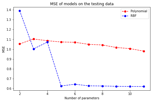
Visually speaking, when the number of RBF kernels grows, the MSE scores of the respective models drop significantly and stay roughly the same if a model has more than 4 basis functions. Combining with the evident results above, it is thereby sensible to choose the linear model with 9 RBF kernels to make predictions.
7 Limitations of Linear Model
Observe that to approximiate a 1-D sine wave function, one can use a linear model with at least 4 basis functions to capture the nonlinearity between one indepedent variable \(x\) and the dependent variable \(y\), which means that more number of indepedent variables may need a myriad of basis functions to adequately express the desired values of the dependent variable. In fact, \(\text{Section } \mathbf{1.4}\) in \(\textbf{Pattern Recognition and Machine Learning}^{[1]}\) illustrates that the oil flow dataset with multidimensional input space requires a great number of coefficients, which is exponentially higher than the number of original input dimensions, to effectively classify the oil type when it comes to using the polynomial model. As a result, to effectively capture the nonlinearity between the input space and the target variable, the number of parameters in a linear model often grows exponentially to the size of the input space, and thus the linear model is prone to the curse of dimensionality. To overcome this, one can use some kind of dimensionality reduction technique to capture the nonlinear manifold of the data, whose dimension is much smaller than the input space, then apply the linear model on this manifold to make predictions, because the information of the manifold is often more efficient to express the dependent variable. Another way is to using more advanced Machine Learning methods with less number of parameters required such as Support Vector Machine, Relevance Vector Machine, or Neural Networks to obtain even better results for either regression or classification tasks.
8 References
[1] Christopher M. Bishop. Pattern Recognition and Machine Learning, Chapter 3.
[2] D.P. Kroese and J.C.C. Chan. Statistical Modeling and Computation, Chapter 7.
[3] MIT lecture notes on MCMC Gibbs Sampling
[4] Oxford lecture notes on Gibbs Sampling
[5] Reversible Markov Chain