Introduction
The goal of this topic is to introduce what does Maximum Likelihood Estimation (MLE) in statistics mean and the application of this method as well as the merits & demerits of this approach.
-
Regarding the first part, the aim is to explain what is the difference between a probability density function and a likelihood function and some live illustrations for likelihood functions.
-
About the second part, it is mainly focused on the most intuitive way to maximize the likelihood function, that is, equating the derivative of the likelihood function to 0 and solving it for the parameters of interest.
-
The third part is about evaluating whether the variance of the estimator for the parameters of interest could achieve the Cramer-Rao lower bound. The motivation behind this task is that the lower variance of the estimator could have, the more likely that the estimated value is closer to the true value).
-
Finally, it is essential to mention MLE for Normal Linear Model since this type of model has a wide variaty of application and it is constituted as the baseline-predictive model before applying other ML algorithms.
Probability Density Function vs Likelihood Function
Suppose that a random variable \(X\) generated from a probability density function (pdf) denoted as \(f(x;\boldsymbol\theta)\), where \(\boldsymbol\theta\) is the parameters of the distribution and everything after the semicolon “;” is treated as known or constant. Therefore, \(f(x;\boldsymbol\theta)\) is a function of \(x\) and everything else is known/fixed.
For instance, if \(f(x;\boldsymbol\theta) = \frac{1}{\sqrt{2\pi\sigma^2}}exp\{-\frac{(x-\mu)^2}{2\sigma^2}\}\), then \(X\) is a random variable generated from the Normal distribution with the corresponding vector of parameters \(\boldsymbol\theta = \begin{pmatrix} \mu \\ \sigma^2 \end{pmatrix}\). Note that, only \(x\) is the variable for the function \(f(x;\boldsymbol\theta)\) in this example.
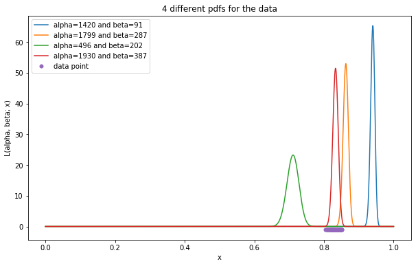
Conversely, the likelihood function treats parameters of a distribution to be unknown variables while the outcome/realization of \(X\) is known. Specifically, the likelihood function is denoted as \(L(\boldsymbol\theta; x)\), which has exactly the same form of \(f(x;\boldsymbol\theta)\). Semantically, the likelihood function tells how “likely” the given data \(x\) is from the distribution with the pdf \(f(x;\boldsymbol\theta)\) and this is often used in the context for the need of determining the hidden/latent distribution (e.g. try computing many pdfs of different distributions to see from which the data is more “likely”). That’s enough for the definition, it’s demo time!
Suppose a random vector \(\mathbf{X} = (X_1, X_2, ..., X_n)^T \sim Beta(\alpha, \beta)\), where \(\alpha\) and \(\beta\) are the parameters for the Beta distribution.
Assume that \(\alpha = 1000\) and \(\beta = 200\) are the true parameters but unknown of Beta distribution for generating the above random vector and the only information given is that the some realizations from \(\mathbf{X}\), which is \(\mathbf{x} = (x_1, x_2, ..., x_{100})^T\) and the data is actually from a Beta distribution. Our job is thus to determine the underlying distribution for the given data, or finding the true values for \(\alpha\) and \(\beta\).
\(\Rightarrow\) The likelihood function for \(\mathbf{x}\) is of the form:
where,
However, the value of \(L(\alpha, \beta; \mathbf{x})\) is extremely small since it is the product of values between 0 and 1 and as the number of observations increases, the value of \(L(\alpha, \beta; \mathbf{x})\) is no longer accurate due to the precision of a float number in computer is 32 bits at maximum. Hence, it is advised to transform the product to the summation by taking the log of \(L(\alpha, \beta; \mathbf{x})\) because \(log\) is a monotonic function in which the increase/decrease in \(L(\alpha, \beta; \mathbf{x})\) also leads to the increase/decrease in \(log(L(\alpha, \beta; \mathbf{x}))\) and vice-versa. Commonly, \(log(L(\alpha, \beta; \mathbf{x}))\) is called log likelihood function and denoted as \(l(\alpha, \beta; \mathbf{x})\).
# Import necessary packages
from scipy.stats import beta
import numpy as np
from matplotlib import pyplot as plt
from celluloid import Camera
import matplotlib.animation as mpl_animation
from scipy import special

writer = mpl_animation.ImageMagickWriter(fps=1) # For animation use

np.random.seed(456)
'''Generate 100 observations from Beta(1000, 200)'''
true_alpha = 1000
true_beta = 200
data = np.random.beta(true_alpha, true_beta, 100)

'''Try many different values of alpha & beta for the pdf
to see which one is the most likely distribution of the given data'''
plt.figure(figsize=(10, 6))
for i in range(4):
    sample_alpha = int(np.ceil(np.random.rand() * 2000)) # Randomly pick a value for alpha starting from 0 to 2000
    sample_beta = int(np.ceil(np.random.rand() * 500)) # Randomly pick a value for beta starting from 0 to 500
    x = np.linspace(0, 1, 1000)
    plt.plot(x, beta.pdf(x, sample_alpha, sample_beta), label='alpha={} and beta={}'.format(sample_alpha, sample_beta))


plt.plot(data, np.zeros(data.shape) - 1, 'o', markersize=5, clip_on=False, label='data point')
plt.xlabel('x')
plt.ylabel('L(alpha, beta; x)')
plt.legend()
plt.title('4 different pdfs for the data')
plt.show()
Maximizing likelihood function
As can be shown in the figure above, the densities of the data points evaluated by the red pdf are generally higher compared to that of other pdf. So it makes more sense to say that those data points are more likely generated from the Beta distribution with \(\alpha = 1929.51\) and \(\beta = 386.99\). Therefore, the approach of MLE is to adjust parameters of a distribution such that it could maximize the likelihood function. Mathematically,
which is equivalent to
Back to the above example, the target is to find out the true parameters for Beta distribution. And based on the given data, the best guess we can make is that the data points should be from the distribution such that their likelihood densities are as large as possible. Consequently, searching for the true parameters for Beta distribution is somehow equivalently to finding out the values that could maximize the likelihood function of Beta distribution.
Recall that the likelihood function of the data has the form of the Equation \(\text{(1)} \Rightarrow\) the log likelihood function of the data should be
The remaining task is to find the value of \(\alpha\) and \(\beta\) that maximize \(l(\alpha, \beta; \mathbf{x})\) so the most straightforward way is by equating the gradient of \(l(\alpha, \beta; \mathbf{x})\) to the vector \(\mathbf{0}\) and solving for \(\alpha\) and \(\beta\). More precisely,
which is equivalent to
where,
Up to this stage, directly solving the Equations \(\text{(2)}\) & \(\text{(3)}\) for \(\alpha\) & \(\beta\) is infeasible due to the fact that these are nonlinear equations. Hence, one of the possible way to find the roots of these equations is using numerical methods. To be specific,
Step 1. Declare the smart-initial values of \(\alpha\) & \(\beta\), which could be derived from the Method of Moment (MoM), that is,
Based on the Law of Large Number (LLN):
\(\begin{cases}
\frac{1}{N}\sum_{i=1}^{N}X_i \to E[X] \\
\frac{1}{N}\sum_{i=1}^{N}X_i^2 \to E[X^2]
\end{cases} \\
\hskip{2em} \text{(as N } \to \infty \text{)} \\
\Rightarrow V[X] \text{ in (4) & (5) }= \frac{1}{N}\sum_{i=1}^{N}X_i^2 - (\frac{1}{N}\sum_{i=1}^{N}X_i)^2\)
\(\rightarrow\) Use \((4)\) & \((5)\) to estimate the initial value of \(\alpha\) & \(\beta\) we get:
where,
Step 2. Choose a numerical method to estimate \(\alpha\) & \(\beta\).
Since taking the 2nd derivative of \(l(\alpha, \beta; \mathbf{x})\) is feasible, it is therefore a reasonable choice to choose \(\text{Newton-Raphson}\) method as a way to find the roots of the Equations \((4)\) & \((5)\) (More detail about why this method works could be found here).
Step 3. Evaluate the 2nd order gradient of \(l(\alpha, \beta; \mathbf{x})\):
where,
Step 4. Define the way to update parameters:
where,
def plot_mle(ax1, ax2, camera, data, theta, iteration):
    '''
        Plot the Equations (2) & (3) given above to demonstrate how Newton-Raphson method helps to find the roots of these functions

        Parameters
        ----------
        ax1: The first axes for sketching the Equation (2)

        ax2: The second axes for sketching the Equation (3)

        camera: An object used to record ax1 and ax2 results

        data: Input data used to compute the Equations (2) & (3)

        theta: The current estimated alpha & beta, which could be referred via the index 0 & 1 of this variable respectively.

        iteration: The current iteration of parameter-updating procedure

        Return
        ------
        NoneType

        Notes
        -----
        Due to limited computational resource, both Equations (2) & (3) can only be plotted in 2D space in which
        The Equation (2) is treated as a one-variable function w.r.t alpha, while beta is assigned to the current estimated value of beta
        Similarly, Equation (3) is treated as a one-variable function w.r.t beta, while alpha is assigned to the current estimated value of alpha
    '''
    partial_l_wrt_alpha = lambda alpha, beta: np.sum(np.log(data)) - (len(data) * special.polygamma(0, alpha)) + (len(data) * special.polygamma(0, alpha + beta))
    partial_l_wrt_beta = lambda alpha, beta: np.sum(np.log(1 - data)) - (len(data) * special.polygamma(0, beta)) + (len(data) * special.polygamma(0, alpha + beta))
    alphas = np.linspace(750, 1500, 1000)
    betas = np.linspace(100, 300, 1000)
    z1 = [partial_l_wrt_alpha(a, theta[1]) for a in alphas]
    z1_at_current_alpha = partial_l_wrt_alpha(theta[0], theta[1])
    z2 = [partial_l_wrt_beta(theta[0], b) for b in betas]
    z2_at_current_beta = partial_l_wrt_beta(theta[0], theta[1])
    ax1.plot(alphas, z1, color='blue')
    ax1.plot(theta[0], z1_at_current_alpha, marker='o', clip_on=False, color='red')
    ax2.plot(betas, z2, color='blue')
    ax2.plot(theta[1], z2_at_current_beta, marker='o', clip_on=False, color='red')
    ax1.set_xlabel('alpha')
    ax1.set_ylabel('Equation (2)')
    ax2.set_xlabel('beta')
    ax2.set_ylabel('Equation (3)')
    ax1.legend(['beta={}, iteration:{}'.format(np.round(theta[1], 2), iteration)])
    ax2.legend(['alpha={}, iteration:{}'.format(np.round(theta[0], 2), iteration)])
    ax1.set_title('Partial derivative of log likelihood w.r.t alpha given beta')
    ax2.set_title('Partial derivative of log likelihood w.r.t beta given alpha')
    camera.snap()
    return
'''Perform MLE to maximize the log likelihood function of Beta distribution'''
fig, (ax1, ax2) = plt.subplots(1, 2, figsize=(10, 6))
camera = Camera(fig)
sample_mean = np.mean(data)
sample_variance = np.var(data)
# Initialize values for alpha & beta
# current_theta[0] is the value of current alpha && current_theta[1] is the value of current beta
current_theta = np.array([((sample_mean ** 2) * (1 - sample_mean) / sample_variance) - sample_mean, \
                          ((sample_mean * (1 - sample_mean) / sample_variance) - 1) * (1 - sample_mean)])
threshold = np.array([1e-5, 1e-5]) # Define the stop condition for updating parameters
# Perform Newton-Raphson method for updating alpha & beta
i = 0 # Memorize the number of iterations
while True:
    plot_mle(ax1, ax2, camera, data, current_theta, i)
    H11 = (len(data) * special.polygamma(1, current_theta[0] + current_theta[1])) - (len(data) * special.polygamma(1, current_theta[0]))
    H12 = len(data) * special.polygamma(1, current_theta[0] + current_theta[1])
    H22 = (len(data) * special.polygamma(1, current_theta[0] + current_theta[1])) - (len(data) * special.polygamma(1, current_theta[1]))
    S1 = (len(data) * special.polygamma(0, current_theta[0] + current_theta[1])) - (len(data) * special.polygamma(0, current_theta[0])) + np.sum(np.log(data))
    S2 = (len(data) * special.polygamma(0, current_theta[0] + current_theta[1])) - (len(data) * special.polygamma(0, current_theta[1])) + np.sum(np.log(1 - data))
    H = np.array([[H11, H12], [H12, H22]])
    S = np.array([S1, S2])
    next_theta = current_theta - np.dot(np.linalg.inv(H), S)
    if (next_theta - current_theta > threshold).all():
        current_theta = next_theta
    else: # If the changes in updated parameters are less than or equal to the threshold, stop the loop
        break
    i += 1
plt.tight_layout()
animation = camera.animate(interval=200)
animation.save('mle_update_parameters.gif', writer=writer)
print('Estimated values of alpha={}, beta={}'.format(int(current_theta[0]), int(current_theta[1])))
Estimated values of alpha=1022, beta=206
'''Plot the pdf of the estimated parameters vs the pdf of the actual parameters'''
x = np.linspace(0, 1, 1000)
plt.figure(figsize=(10, 6))
plt.plot(x, beta.pdf(x, current_theta[0], current_theta[1]), color='red', label='MLE pdf with alpha={} and beta={}'.format(int(current_theta[0]), int(current_theta[1])))
plt.plot(x, beta.pdf(x, true_alpha, true_beta), color='blue', label='true pdf with alpha={} and beta={}'.format(true_alpha, true_beta))
plt.plot(data, np.zeros(data.shape) - 1, 'o', markersize=5, clip_on=False, label='data point')
plt.xlabel('x')
plt.ylabel('f(x; alpha, beta)')
plt.legend()
_ = plt.title('Actual pdf vs pdf with parameters derived from MLE')
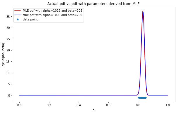
With only 2 iterations from Newton-Raphson algorithm, the near-optimal solution for the log likelihood function can be easily obtained. This is due to the fact that the initial values of \(\alpha\) & \(\beta\) could be evaluated analytically using MoM; as a result, the initial values are almost close to the MLE solution.
So far, the parameters derived from MLE reflects the pdf (in red) which is almost analogous to the true pdf (in blue) as shown in the figure above. Hence, the more data could be obtained, the more accurate MLE method could achieve.
It is noteworthy that, some likelihood functions are intractable to take derivative or to solve for the parameters of interest, but having said that, those problems could be tackled by using some numerical methods which shall be further discussed here.
Cramér-Rao Information Inequality
The purpose of the C-R inequality is to evaluate whether the variance of the estimator could achieve the C-R lower bound (CRLB). This is particularly useful if we want to compare the performance of many estimators (e.g. the closer of the variance’s estimator to the CRLB, the better the estimator is). More reasons could be found here.
In this section, we shall not discuss the way to assess whether the MLE estimator of Beta distribution achieve CRLB since there is no closed-form solution for estimating \(\alpha\) & \(\beta\) as shown above; in other words, one of the numerical methods was used to compute MLE estimation of \(\alpha\) & \(\beta\). Even the estimated values of \(\alpha\) & \(\beta\) have the analytical solution obtained via MoM, evaluating the variance and the expectation of these estimations are still intractable.
Therefore, it is better to set another example to demonstrate how CRLB works.
Suppose a random vector \(\mathbf{X} = (X_1, X_2, ..., X_n)^T \overset{iid}{\sim} \mathcal{N}(\mu, \sigma^2)\)
Given the fact that the vector \(\mathbf{x} = (x_1, x_2, ..., x_{N})^T\) is one realization of the vector \(\mathbf{X}\)
\(\Rightarrow\) The MLE estimator of \(\mu\), which could be obtained by solving the derivative of \(l(\mu, \sigma^2; \mathbf{x})\) w.r.t \(\mu\), is going to be:
Similarly, the MLE estimator of \(\sigma^2\) is of the form:
However, the \(\hat{\sigma}^2\) above is a biased estimator, that is, \(E[\hat{\sigma}^2] \neq \sigma^2\)
Proof:
Consider \((6)\):
Consider \((7)\):
Now, let us examine whether the variance of these estimators could achieve the CRLB.
Regarding the definition of Cramér-Rao Information Inequality, it states that the variance of an estimator \(Var(T(\mathbf{X}))\) for estimating the parameter \(\boldsymbol\theta\) is greater than or equal to \(\nabla g(\boldsymbol\theta)^T I(\boldsymbol\theta)^{-1} \nabla g(\boldsymbol\theta)\). Formally,
where,
The proof of CRLB is quite straightforward. It is thus easier to mention about the idea of the proof only as well as a good way to remember this definition.
Proof (Sketch):
Consider \(\theta\) in 1-D case, denote the derivative of the log likelihood function as \(S(\theta) = d\frac{l(\theta; \mathbf{x})}{d\theta}\), aka the score function, and \(T(\mathbf{x})\) as the estimator of the parameter \(\theta\).
Knowing the fact that the Pearson correlation of \(S(\theta)\) & \(T(\mathbf{x})\) is between -1 and 1. Specifically,
It remains to show that \(Cov(S, T)\) is indeed the derivative of \(g(\theta) = E[T(\mathbf{x})]\) w.r.t \(\theta\) under regularity condition (Hint: \(Cov(S, T) = E[ST] - \underbrace{E[S]}_{0}E[T]\)). Consequently,
CRLB for the estimator of \(\mu\): \(\hat{\mu} = \frac{\sum_{i=1}^{N}x_i}{N}\)
Since \(\mathbf{x} \overset{iid}{\sim} \mathcal{N}(\mu, \sigma^2) \Rightarrow l(\mu, \sigma^2; \mathbf{x}) = -\frac{N}{2}ln(2\pi) -\frac{N}{2}ln(\sigma^2) - \sum_{i=1}^{N}\frac{(x_i - \mu)^2}{2\sigma^2}\)
\(\rightarrow\) Taking the expectation of \(\hat{\mu} = T(\mathbf{x})\) w.r.t \(\mu\) yields:
\(\Rightarrow T(\mathbf{x}) \text{ is an unbiased estimator of } \mu\)
- Proof for \((\star) == \mu\):
\(\rightarrow\) Using the Moment Generating Function (MGF) of \(X\) gives:
\((8), (9) \Rightarrow\)
\(\Rightarrow\) The estimator \(\hat{\mu}\) of \(\mu\) attains CRLB.
CRLB for the estimator of \(\sigma^2\): \(\hat{\sigma}^2 = s^2 = \frac{\sum_{i=1}^{N}(x_i - \bar{x})^2}{N-1}\)
\(\cdot \begin{cases} \frac{dl(\mu, \sigma^2; \mathbf{x})}{d\sigma^2} = -\frac{N}{2\sigma^2} + \frac{\sum_{i=1}^{N}(x_i - \mu)^2}{2(\sigma^2)^2} \\ \frac{d^2l(\mu, \sigma^2; \mathbf{x})}{d(\sigma^2)^2} = \frac{N}{2(\sigma^2)^2} - \frac{\sum_{i=1}^{N}(x_i-\mu)^2}{(\sigma^2)^3} \\ E[\hat{\sigma}^2] = g(\sigma^2) = \sigma^2 \end{cases}\)
According to CRLB definition:
- Note that the term \(\frac{(N-1)s^2}{\sigma^2} \sim \chi_{N-1} \Rightarrow Var(\frac{(N-1)s^2}{\sigma^2}) = \frac{(N-1)^2}{(\sigma^2)^2}Var(s^2) = 2(N-1)\)
\((10), (11) \Rightarrow\)
Hence, \(\hat{\sigma}^2 = s^2\) does NOT attain CRLB even it is the unbiased estimator.
MLE for Normal Linear Model
Introduction to Linear Model
When it comes to Linear Model, it is not only about representing a linear combination of linear functions (e.g. \(f(x_1, x_2, x_3) = ax_1 + bx_2 + cx_3 + d\)), but also introducing a model with multiple nonlinear functions with associated adjustable parameters (e.g. \(f(x_1, x_2, x_3) = ax_1 + bsin(x_2) + cx_3^5 + d\)).
The big plus of Linear Model is the fact that it could utilize many useful class of functions by taking linear combinations of fixed set of nonlinear functions of the input variables/predictors, aka basis functions. What is more, since the model itself explicitly restricts the relationship of indepedent variables to be linear, it is hence easy to interpret the influence of predictors as well as giving some simple but nice analytical properties such as finding optimal parameters for the model could be addressed analytically by Least Squares approach, and relationship between predictors could be transformed from nonlinear into linear by nonlinear functions.
However, the number of parameters in Linear Model is fixed and manually defined, which could be insufficient to capture some real world problems requiring thounds of parameters or more.
Mathematically, the form of Linear Model could be defined as
where,
\(N\) is the number of observations and \(d\) is the number of parameters/predictors of this model.
\(\phi_j(\mathbf{x}_i)\) is the jth basis function which takes the ith observation as the input.
For every \(x_{i\cdot}\), it could be understood as the ith observation.
- A typical example of Linear Model is Polynomial regression. For instance, \(y = \beta_0 + \beta_1x + \beta_2x^2 + \beta_3x^3 + \ldots + \beta_dx^d\). Note that this formula is only accountable for one realization at a time
\(\rightarrow\) The formula for Polynomial regression of multiple records could be represented in matrix form as follows
Normal Linear Model
Regarding Normal Linear Model, it is nothing but of the form of Linear Model and assumes that the outcomes have the noise follows Normal distribution with the mean \(\boldsymbol\mu_{\text{noise}} = \mathbf{0}\) and the covariance matrix \(\Sigma\). Mathematically,
where,
For simplicity, we shall treat the noise of all records follows an isotropic Gaussian distribution. That is, \(\boldsymbol\epsilon \sim \mathcal{N}(\mathbf{0}, \sigma^2\mathbf{I})\) (e.g. every record has the same variance \(\sigma^2\) and independent from each other).
Moving onto MLE approach, given a training data set with \(N\) observations in which each observation \(i\) has its feature vector \(\boldsymbol\phi(\mathbf{x}_i)\) associated with an outcome \(y_i\). The goal is to find the most sensible set of parameters \(\boldsymbol\beta\) and \(\sigma^2\) associated with the model and the data repsectively that maximizes the likelihood functions for all given data points. In other words, we wish to find
It is worth mentioning that the noise of data follows a multivariate Normal distribution based on the definition of Normal Linear Model, the outcomes of observations \(\mathbf{y} = \begin{pmatrix} y_1 \\ \vdots \\ y_N \end{pmatrix}\) are therefore the linear transformation of \(\mathcal{N}(\mathbf{0}, \sigma^2\mathbf{I})\), which also can be modelled as a multivatiate Normal distribution with mean \(\mathbf{X}\boldsymbol\beta\) and covariance matrix \(\sigma^2\mathbf{I}\), where \(\mathbf{X} = \begin{pmatrix} \boldsymbol\phi(\mathbf{x}_1)^T \\ \vdots \\ \boldsymbol\phi(\mathbf{x}_N)^T \end{pmatrix}\). Hence, the product of likelihood functions of the data can also be defined as
Note that the logarithm function is a non-decreasing function; therefore, maximizing the logarithm of \(f(\mathbf{y}|\boldsymbol\beta, \mathbf{X}, \sigma^2)\) is equivalent to maximizing the likelihood function itself. Mathematically speaking,
To find the value of \(\boldsymbol\beta\) that maximizes \((12)\), setting the derivative of \((12)\) w.r.t \(\boldsymbol\beta\) to \(\mathbf{0}\) and solving for \(\boldsymbol\beta\) is one of the most intuitive way. More precisely, define
where,
\(\hskip{5em} L_D(\boldsymbol\beta) = \frac{1}{2}\sum_{i=1}^{N}(y_i - \boldsymbol\beta^T\boldsymbol\phi(\mathbf{x}_i))^2\) is the summation of squares error between \(\mathbf{y}\) & \(\mathbf{X}\boldsymbol\beta\) over all given data points in \(D\)
\(\hskip{5em} \boldsymbol\phi(\mathbf{x}_i) = \begin{pmatrix} \phi_1(\mathbf{x}_i) \\ \phi_2(\mathbf{x}_i) \\ \vdots \\ \phi_d(\mathbf{x}_i) \end{pmatrix} \space\) is the vector of basis functions
Note that the function \(L_D(\boldsymbol\beta)\) is of the form of the least squares function. Therefore, it is equivalent to say that searching for optimal parameters by MLE approach is similar to optimizing parameters by least squares method.
Another way to obtain the optimal \(\boldsymbol\beta\) for \(L_D(\boldsymbol\beta)\) is to view this problem in terms of a geometry argument. Specifically, we want to find \(\boldsymbol\beta\) such that \(\mathbf{X}\boldsymbol\beta\) is as close to \(\mathbf{y}\) as possible with fixed \(\mathbf{X}\). In geometrical perspective, the closest \(\mathbf{X}\boldsymbol\beta\) to \(\mathbf{y}\) is indeed the the projection of \(\mathbf{y}\) onto the vector space \(\mathbf{X}\). For the ease of interpretation, the image below illustrates why \(\mathbf{X}\boldsymbol\beta = \text{proj}_{\mathbf{X}}(\mathbf{y})\) is the closest distance between \(\mathbf{y}\) and \(\mathbf{X}\boldsymbol\beta\).
\(\hskip{10em}\)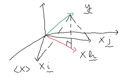
Consequently, the solution for \(\mathbf{X}\boldsymbol\beta\), where \(L_D(\boldsymbol\beta)\) is minimized, should be \(\mathbf{Xh}\).
To be specific,
\(\rightarrow\) If \(\mathbf{h}\) is used as the solution for \(\boldsymbol\beta\), this result is equivalent to \(\boldsymbol\beta_{\text{MLE}}\) acquired via solving \(\nabla L_D(\boldsymbol\beta) = \mathbf{0}\) for \(\boldsymbol\beta\).
Next, to optimize for \(\sigma^2\), setting the derivative of \((12)\) w.r.t \(\frac{1}{\sigma^2}\) to 0 and solving for \(\frac{1}{\sigma^2}\) results in:
Regularized least squares
Even the solution obtained by least squares method is an easy-intuitive way, there is still a pitfall in estimating \(\boldsymbol\beta\) by MLE approach, that is, the model could be overfitting if the it is trained with relatively small data set since the objective is to maximize the likelihood of every observation, which could possibly be heavily influenced by the outliers and adapted to the noise as well. Thereby, one of the most sensible manner is to add another term to the sum-of-squares error function to control overfitting issue, which is so-called regularization term. In particular, the new objective function now becomes
where
\(\hskip{5em} L_D(\boldsymbol\beta)\) is a data-dependent error function already defined above.
\(\hskip{5em} L_{\boldsymbol\beta}(\boldsymbol\beta)\) is the regularization term, which serves as the purpose of shrinking model’s parameters towards zero unless supported by the data.
Generally, the regularizer takes the form
\(\rightarrow\) Since the regularizer depends on the value of \(\lambda\); hence, minimizing \((13)\) is identical to finding values for \(\boldsymbol\beta\) to reduce the influence of \(\lambda\) in order to make the whole expression as minimal as possible. For example, the loss function could be
However, the values for hyperparameters \(\lambda\) and \(q\) are manually defined, the issue thus becomes tuning hyperparameters \(\lambda\) and \(q\). The way of selecting values for those hyperparameters to construct a good-fit model would be shortly discussed in the following part.
For the case of Normal Linear Model, the sum-of-squares error function \(L_D(\boldsymbol\beta)\) is a quadratic function of \(\boldsymbol\beta\); hence, choosing \(q=2\) for the regularizer would make the total error function remain a quadratic function of \(\boldsymbol\beta\) as same as the previous example. To be exact, the total error function with \(q=2\) has the following form
\(\rightarrow\) Setting the the gradient of the equation \((14)\) to \(\mathbf{0}\) and solving for \(\boldsymbol\beta\) gives
In fact, the method of searching for the optimal solution for \((14)\) is similar to using Lagrange multipliers for maximizing/minimizing the function \(L_D(\boldsymbol\beta)\) subject to the constraint \(\sum_{i=1}^{N}|\beta_i|^q \leqslant \eta\) for an appropriate value of the parameter \(\eta\).
That’s enough for maths. Let’s work on an example to see how regularization helps MLE approach avoid overfitting problem!
''' Generate some data from a 2nd-degree polynomial model with the noise followed a Normal distribution '''
train_sample_size = 100
test_sample_size = 20
noise_std = 100
true_beta_0 = 2.5
true_beta_1 = 7.89
true_beta_2 = 4.56
true_beta = np.array([true_beta_0, true_beta_1])

data_x = np.random.rand(train_sample_size + test_sample_size)
data_y = true_beta_0 + (true_beta_1 * data_x) + np.random.normal(loc=0, scale=noise_std, \
                                                                size=train_sample_size + test_sample_size)
data_x_train, data_x_test = data_x[:train_sample_size], data_x[train_sample_size:]
data_y_train, data_y_test = data_y[:train_sample_size], data_y[train_sample_size:]
def lm_cross_validation(data_X, data_y, k_folds, lmbda):
    '''
        Perform k-fold cross validation for Linear Model with Ridge regression
        and compute the average sum of squared errors throughout k scenarios

        Parameters
        ----------
        data_X: Input of data, which are also considered as the features of data

        data_y: Output of data, which is also known as the outcome of data

        k_folds: Number of folds for cross validation procedure

        lmda: The hyperparameter of regularization term

        Return
        ------
        FloatType: The average sum of squared errors for k subsamples

        Notes
        -----
        For more information why cross validation helps in finding good values for hyperparameters tuning,
        refer to this link -> https://medium.com/datadriveninvestor/k-fold-cross-validation-for-parameter-tuning-75b6cb3214f

    '''
    subsample_size = int(np.ceil(len(data_X) / k_folds))
    avg_total_squares_error = 0
    for k in range(k_folds):
        test_indices = [i + k*subsample_size for i in range(subsample_size)] if k + 1 < k_folds \
                        else [i + k*subsample_size for i in range(len(data_X) - (k*subsample_size))]

        X_train, y_train = np.delete(data_X, test_indices, axis=0), np.delete(data_y, test_indices, axis=0)

        X_test = data_X[k*subsample_size:(k*subsample_size + subsample_size)] \
                        if k + 1 < k_folds else data_X[k*subsample_size:]
        y_test = data_y[k*subsample_size:(k*subsample_size + subsample_size)] \
                        if k + 1 < k_folds else data_y[k*subsample_size:]
        # Compute the value for total error function
        beta_hat = np.dot(np.dot(np.linalg.inv((np.eye(data_X.shape[1]) * lmbda) + np.dot(X_train.T, X_train)), X_train.T), y_train)
        Xbeta_test = np.dot(X_test, beta_hat)
        avg_total_squares_error += ((1/2) * np.dot((y_test - Xbeta_test).T, (y_test - Xbeta_test))) + \
                                ((1/2) * np.dot(beta_hat.T, beta_hat))

    return avg_total_squares_error / k_folds
''' MLE for Normal Linear Model for unregularized total error function '''
# Suppose that the hypothesized model is also a 2nd-degree polynomial model.
X = np.dstack((np.ones(train_sample_size), data_x_train))[0]
y = data_y_train
mle_unregularized_beta = np.dot(np.dot(np.linalg.inv(np.dot(X.T, X)), X.T), y)
''' MLE for Normal Linear Model for regularized total error function '''
# Suppose that the hypothesized model is also a 2nd-degree polynomial model.
best_lmbda, best_score = 2, 9999999 # Initialize values for best_lmbda, best_score
lmbda_space = np.logspace(-5, 5, 10000) # Domain of lmbda
n_iter = 460 # There is 99% chance that one candidate will be selected from the best 1% candidates in the given lmbda space
k_folds = 4 # Declare number of folds for cross validation procedure
# Perform randomized grid search method for picking good value of lmbda
for i in range(n_iter):
    selected_lmbda = np.random.choice(lmbda_space)
    score = lm_cross_validation(X, y, k_folds, selected_lmbda)
    if score < best_score:
        best_lmbda = selected_lmbda
        best_score = score

mle_regularized_beta = np.dot(np.dot(np.linalg.inv((best_lmbda*np.eye(X.shape[1])) + np.dot(X.T, X)), X.T), y)
''' Plot the graph of Normal Linear Models with & without regularized total error function on training data '''
x_range = np.linspace(np.min(X[:, 1]) - 1, np.max(X[:, 1]) + 1, 10000)
X_range = np.dstack((np.ones(10000), x_range))[0]
y_unregularized_range = np.dot(X_range, mle_unregularized_beta)
y_regularized_range = np.dot(X_range, mle_regularized_beta)
y_true_range = np.dot(X_range, true_beta)

plt.figure(figsize=(10, 6))
plt.plot(x_range, y_unregularized_range, color='blue', label='Model with regularization-free')
plt.plot(x_range, y_regularized_range, color='red', label='Model with regularization')
plt.plot(x_range, y_true_range, color='green', label='True linear model')
plt.plot(data_x_train, data_y_train, '+', markersize=5, clip_on=False, label='Data point')
plt.title('Visualization of unregularized linear model vs regularized linear model optimized by MLE')
plt.xlabel('x')
plt.ylabel('y')
plt.legend()
plt.show()

# Compute the total squared errors with testing data to see which model performs better
X_test = np.dstack((np.ones(len(data_x_test)), data_x_test))[0]
score_unregularized_model = np.dot((data_y_test - np.dot(X_test, mle_unregularized_beta)).T, \
                                           data_y_test - np.dot(X_test, mle_unregularized_beta))
score_regularized_model = np.dot((data_y_test - np.dot(X_test, mle_regularized_beta)).T, \
                                           data_y_test - np.dot(X_test, mle_regularized_beta))
print('Sum-of-squares value for unregularized model: {}'.format(score_unregularized_model))
print('Sum-of-squares value for regularized model: {}'.format(score_regularized_model))
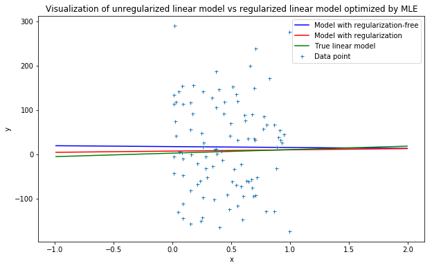
Sum-of-squares value for unregularized model: 299335.89017885574
Sum-of-squares value for regularized model: 289619.40085747186
As can be seen from the illustration above, the model with regularization term tends to approximate much better and have smaller sum-of-squares value compared to that of the model with unregularized cost function.
For more information why minimizing regularized total error function results in better approximation. Let’s look at the contour plot of unregularized total error function w.r.t \(\beta_0\) & \(\beta_1\) and the constraint defined by regularization term to see the feasible domain of solution.
'''Contour plot for unregularized total error function subject to the constraint defined by regularization term'''
# Since the constraint defined by regularization term is of the form of a circle equation
# And the solution must be the tangent of both total error function and the constraint function
# Hence, the radius where the constraint function meets the total error function should be sqrt(beta_0^2 + beta_1^2)
constraint_radius = np.sqrt((mle_regularized_beta[0] ** 2) + (mle_regularized_beta[1] ** 2))

# Initialize mesh points for drawing contour plot of unregularized total error function
mesh_size = 100
beta_0 = np.linspace(-50, 50, mesh_size)
beta_1 = np.linspace(-50, 50, mesh_size)
Beta_0, Beta_1 = np.meshgrid(beta_0, beta_1)

total_error_function = np.eye(mesh_size) # Initialize values for total_error_function
for i in range(mesh_size):
    for j in range(mesh_size):
        beta = np.array([Beta_0[i, j], Beta_1[i, j]])
        Xbeta = np.dot(X, beta)
        total_error_function[i, j] = (1/2) * np.dot((y - Xbeta).T, (y - Xbeta))

sse_for_regularized_beta = (1/2) * np.dot((y - np.dot(X, mle_regularized_beta)).T, (y - np.dot(X, mle_regularized_beta)))
sse_for_unregularized_beta = (1/2) * np.dot((y - np.dot(X, mle_unregularized_beta)).T, \
                                            (y - np.dot(X, mle_unregularized_beta))) + 100

fig, ax = plt.subplots(figsize=(10, 6))

circle = plt.Circle((0, 0), constraint_radius, color='blue', fill=False)
ax.add_artist(circle)

cost_function_contour = ax.contour(Beta_0, Beta_1, total_error_function, \
           [sse_for_unregularized_beta, sse_for_regularized_beta, 555000, 585000, 700000], colors='red')

optimal_beta, = ax.plot(mle_regularized_beta[0], mle_regularized_beta[1], 'o', markersize=5, color='green')

contour_legend, _ = cost_function_contour.legend_elements()

ax.set_xlim((-50, 50))
ax.set_ylim((-50, 50))
ax.set_xlabel('beta_0')
ax.set_ylabel('beta_1')
ax.legend((contour_legend[0], circle, optimal_beta), ('contour lines for total error function', \
                                                         'regularization constraint', \
                                                         'optimal beta'))
ax.set_title('Contour plot for unregularized total error function and regularization constraint')
plt.show()
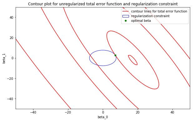
So far, introducing regularization term is a great way to overcome severe overfitting problem by MLE approach, although choosing the sensible model (e.g selecting basis functions for Normal Linear Model) is generally more important since it reflects the overal behaviour of the model for a particular problem. For the next topic, we shall discuss the Bayesian treatment of linear regression and the reasons for choosing this approach over MLE fashion.
Reference
[1] Christopher M. Bishop. Pattern Recognition and Machine Learning, Section 3.1, Chapter 3.
[2] D.P. Kroese and J.C.C. Chan. Statistical Modeling and Computation, Chapter 6.
[3] Fisher Information and Cramér-Rao Bound.