Motivation
When it comes to clustering, there are many well-known unsupervised algorithms that could categorize the given data into many sensible groups, namely, K-mean & Hirarchical clustering algorithms. Yet, those mentioning algorithms tend to assign each individual into a single group, which is not always the case for real-world scenario; for instance, an individual could follow two religious belief at the same time. What is more, the overlapping between clusters is not possible. Hence, Gaussian Mixture Model (GMM) with the help of Expectation Maximization (EM) algorithm is an initiative to address the aforementioned issues. More precisely, this article is going to cover the mathematical derivation and the implementation with regard to GMM optimized by EM algorithm as well as the comparison between the performance of GMM vs that of K-mean algorithm. More than that, the mathematical relation between GMM and K-Means will also be illustrated later in order to explain why GMM is able to accommodate the limitation of K-Means algorithm in terms of clustering.
Mathematical Concept & Implementation of GMM using EM algorithm
Gaussian Mixture Model definition
Suppose that \(X\) is a random variable that is generated from either one of the 3 groups, where each group is Gaussian distributed with its mean \(\boldsymbol\mu\) and covariance \(\Sigma\). Mathematically, \(X\) could be presented as follows:
where,
$$\pi_z$$ is the prior probability that a random variable $$X$$ could possibly be Gaussian distributed with $$\mathcal{N}(\boldsymbol\mu_z, \Sigma_z)$$, which corresponds to the class/cluster $$z$$.
And $$\pi_1, \pi_2, $$ and $$\pi_3$$ are under the constraint: $$\pi_1 + \pi_2 + \pi_3 = 1$$
Initialize data points for the corresponding clusters
Suppose that the distribution of a data point can be expressed as follows:
where,
\(\Rightarrow\) The procedure to generate samples corresponding to the given distribution can be described in the following 2 steps:
- The cluster \(C_i\) to which the new data point \(X_i\) will be assigned can be simulated by
$$C_i \sim Multinomial(N=1, \boldsymbol{p} = (0.5, 0.25, 0.25))$$ - Update the data for the data point \(X_i\) from the appropriate distribution, whose class should be equivalent to the class assigned to \(X_i\) given in Step 1 via
$$X_i \sim \mathcal{N}(\boldsymbol{\mu}_{C_i}, \boldsymbol{\Sigma}_{C_i})$$
## Importing necessary packages
import numpy as np
import matplotlib.pyplot as plt
from celluloid import Camera # For animation use
import matplotlib.animation as mpl_animation # For animation use

writer = mpl_animation.ImageMagickWriter(fps=1) # For animation use
## Define the distribution of cluster 1, 2, and 3
mus = np.array([
    [2, 8],
    [5, 6],
    [1, 2]
])

sigmas = np.array([
    [
        [2, 1.6],
        [1.6, 2]
    ],
    [
        [1, 0.5],
        [0.5, 1]
    ],
    [
        [3, 1.2],
        [1.2, 3]
    ]

])

pis = np.array([0.5, 0.25, 0.25])

true_theta = {'mu': mus, 'sigma': sigmas, 'pi': pis}
## Generate data
N = 10000 # Number of data points to be generated from the given clusters
N_FEATURES = 2 # Number of features for an example
data = np.zeros((N, N_FEATURES))
labels = np.zeros(N)
for i in range(N):
    labels[i] = np.where(np.random.multinomial(n=1, pvals=np.array([pis[0], pis[1], pis[2]])) == 1)[0]
    cluster_i = int(labels[i])
    data[i, :] = np.random.multivariate_normal(mean=mus[cluster_i], cov=sigmas[cluster_i])
## Visualize the generated data points
cluster_1_idx = np.where(labels == 0)
cluster_2_idx = np.where(labels == 1)
cluster_3_idx = np.where(labels == 2)
_ = plt.scatter(x=data[cluster_1_idx, 0], y=data[cluster_1_idx, 1], c='red', marker='^')
_ = plt.scatter(x=data[cluster_3_idx, 0], y=data[cluster_3_idx, 1], c='green', marker='*')
_ = plt.scatter(x=data[cluster_2_idx, 0], y=data[cluster_2_idx, 1], c='blue', marker='o')
_ = plt.xlabel('x1')
_ = plt.ylabel('x2')
_ = plt.title('Visualization of all data points and their corresponding class/cluster')
_ = plt.show()
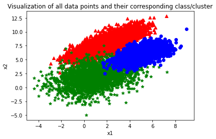
As can be seen from the graph above, there are overlappings in between cluster 1, 2, and 3 and the covariance as well as the variation of each class are highly distinct.
Define initial values for the parameters associated with the proposal Gaussian Mixture Model
Suppose the labels for the generated dataset above are unknown. Specifically,
## Visualize the generated data points
cluster_1_idx = np.where(labels == 0)
cluster_2_idx = np.where(labels == 1)
cluster_3_idx = np.where(labels == 2)
_ = plt.scatter(x=data[cluster_1_idx, 0], y=data[cluster_1_idx, 1], c='blue', marker='o')
_ = plt.scatter(x=data[cluster_3_idx, 0], y=data[cluster_3_idx, 1], c='blue', marker='o')
_ = plt.scatter(x=data[cluster_2_idx, 0], y=data[cluster_2_idx, 1], c='blue', marker='o')
_ = plt.xlabel('x1')
_ = plt.ylabel('x2')
_ = plt.title('Visualization of all unlabeled data points')
_ = plt.show()
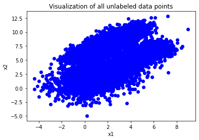
Assume that those data points are generated from 3 clusters in which their distribution follows a particular Gaussian Mixture Model, which is of the form of the Equation \(\text{(1)}\). Therefore, our first step is to randomly assign values for the parameters of the proposal model, which could be demonstrated by the following lines of code.
## Initialize values for model's parameters
est_mus = np.array([
    [1, 1],
    [2, 2],
    [3, 3]
]).astype(float)
est_sigmas = np.array([
    [
        [1, 0.5],
        [0.5, 1]
    ],
    [
        [1, 0.5],
        [0.5, 1]
    ],
    [
        [1, 0.5],
        [0.5, 1]
    ]
]).astype(float)

est_pis = np.array([0.2, 0.1, 0.7])

prev_theta = {'mu': est_mus, 'sigma': est_sigmas, 'pi': est_pis}
Define the log likelihood function for the proposal model
def ln_likelihood(X, theta):
    '''
        This function takes the log of the likelihood function of Gaussian Mixture Model (GMM) for all given data

        Parameters
        ----------
        X: features' values of all instances in the given dataset

        theta: the input dictionary containing all necessary parameters for the GMM

        Returns
        -------
        Log likelihood of GMM
    '''
    def multivariate_normal_pdf(x, mu, sigma):
        '''
            This is a helper function, which calculates the pdf of multivariate normal distribution with mean mu
            and covariance matrix sigma
        '''
        normalizing_const = (1 / ((2 * np.pi) ** (mu.shape[0] / 2))) * \
                            (np.linalg.det(sigma) ** (-0.5))
        return np.exp((-0.5) * (x - mu).T @ np.linalg.inv(sigma) @ (x - mu)) * normalizing_const
    llh = 0
    for x_i in X: # Iterate through every example
        lh = 0
        for z in range(len(theta['mu'])): # Compute the likelihood of the examining example with respect to a specific class
            lh += theta['pi'][z] * multivariate_normal_pdf(x_i, theta['mu'][z], theta['sigma'][z])
        llh += np.log(lh)
    return llh
# An example of how to use ln_likelihood function
ln_likelihood(data, {'mu': est_mus, 'sigma': est_sigmas, 'pi': est_pis})
-152672.48693508524
Define the conditional distribution of the latent variable \(Z\) and the expectation of log complete-data likelihood \(Q(\boldsymbol{\theta}_{t-1}, \boldsymbol{\theta}_{t})\)
Since the EM algorithm requires the specification of the complete-data likelihood distribution and the associated variable \(z\) depicting which group/cluster a data point belongs to, and the data is assumed to follow a Gaussian Mixture Model, the complete-data likelihood is essentially:
- Explain:
\(\Rightarrow\) the log complete-data likelihood is basically:
\(\Rightarrow\) In general, the log complete-data likelihood for N data points can be viewed as:
The next step is to specify \(Q(\theta_{t-1}, \theta_t)\), which is nothing but the expected value of log complete-data likelihood with respect to the conditional distribution of \(Z \sim f(z|\boldsymbol{\theta}_{t-1}, x)\):
def complete_data_likelihood(z, x, theta):
    '''
        This function evaluates the complete-data likelihood function for a single data point,
        which is of the form of Equation (2)

        Parameters
        ----------
        z: the observable value of variable Z

        x: features' values of the data point

        theta: the input dictionary containing all necessary parameters for the proposal model

        Returns
        -------
        Density of L(theta|x, z)
    '''
    pi = theta['pi'][z]
    mu = theta['mu'][z]
    sigma = theta['sigma'][z]
    return pi * (np.linalg.det(sigma) ** (-0.5)) * \
            ((2 * np.pi) ** (-mu.shape[0] / 2)) * \
            np.exp(-0.5 * (x - mu).T @ np.linalg.inv(sigma) @ (x - mu))

def g(z, x, theta):
    '''
        This function computes the conditional distribution of latent variable Z given x and theta

        Parameters
        ----------
        z: the value of interest of variable Z

        x: features' values of the data point

        theta: the input dictionary containing all necessary parameters for the proposal model

        Returns
        -------
        Density of g(z)
    '''
    normalizing_const = 0
    numerator = complete_data_likelihood(z, x, theta) # Density of the conditional dist of z given x and theta
    for c in range(len(theta['pi'])): # Iterate through every possible class
        normalizing_const += complete_data_likelihood(c, x, theta)
    return numerator / normalizing_const
# Some examples for using complete_data_likelihood, and g functions
complete_data_likelihood(2, np.array([0.2, 5]), {'mu': est_mus, 'sigma': est_sigmas, 'pi': est_pis})
g(2, np.array([0.2, 5]), {'mu': est_mus, 'sigma': est_sigmas, 'pi': est_pis}) + \
g(1, np.array([0.2, 5]), {'mu': est_mus, 'sigma': est_sigmas, 'pi': est_pis}) + \
g(0, np.array([0.2, 5]), {'mu': est_mus, 'sigma': est_sigmas, 'pi': est_pis})
1.0
Derive the way to update \(\boldsymbol{\theta}_t\) based on previous set of parameters \(\boldsymbol{\theta}_{t-1}\) so as to maximize \(Q(\boldsymbol{\theta}_{t-1}, \boldsymbol{\theta}_t)\)
Update \(\boldsymbol{\mu}_z^{(t)}\)
Since the goal is to maximize \(Q(\boldsymbol{\theta}_{t-1}, \boldsymbol{\theta}_t)\), which is equivalent to maximizing the likelihood function of the Gaussian Mixture Model (check out \(\textbf{Appendix: Mathematical Concept of EM algorithm}\) for having a better intuition why maximizing \(Q(\boldsymbol{\theta}_{t-1}, \boldsymbol{\theta}_t)\) is equivalent to maximizing the marginal likelihood function \(L(\boldsymbol{\theta} | \mathbf{x})\)). Thus, setting the derivative of \(Q(\boldsymbol{\theta}_{t-1}, \boldsymbol{\theta}_t)\) with respect to \(\boldsymbol{\mu}_z^{(t)}\) to \(\mathbf{0}\) and solving for \(\boldsymbol{\mu}_z^{(t)}\) yields:
Recall that,
Update \(\Sigma_z^{(t)}\)
Similarly, setting the derivative of the Equation \(\text{(6)}\) with respect to \((\boldsymbol{\Sigma}_z^{(t)})^{-1}\) to \(\mathbf{0}\) and solving for \(\boldsymbol{\Sigma}_z^{(t)}\) yields:
Given that \(Q(\boldsymbol{\theta}_{t-1}, \boldsymbol{\theta}_t)\) can also be expressed in the following form:
Update \(\pi_z^{(t)}\)
Lastly, maximizing the Equation \(\text{(4)}\) or \(\text{(6)}\) with respect to \(\pi_z^{(t)}\) and subjecting to the constraint \(\pi_1^{(t)} + \pi_2^{(t)} + \pi_3^{(t)} = 1\) is the step to update \(\pi_z\). Thus, solving for \(\pi_z^{(t)}\) gives:
def update_parameters(z, X, prev_theta):
    '''
        This function computes the mean, covariance as well as the distribution of the given class z based on data
        and previous values of the same set of parameters

        Parameters
        ----------
        z: the associated class for the parameter of interest

        X: features' values of the dataset

        prev_theta: the input dictionary containing all necessary parameters for the proposal model previously

        Returns
        -------
        Updated mean, covariance, and pi parameters
    '''
    mu_numerator = np.zeros(X.shape[1])
    g_z = np.zeros(X.shape[0]) # Store all g_i(z) values
    sum_g_z = 0
    for i, x_i in enumerate(X):
        g_i_z = g(z, x_i, prev_theta) # g_i(z)
        g_z[i] = g_i_z
        mu_numerator += x_i * g_i_z
        sum_g_z += g_i_z
    ## Compute the new mu
    new_mu = mu_numerator / sum_g_z
    ## Compute the new pi
    new_pi = sum_g_z / X.shape[0]
    ## Compute the new sigma
    sigma_numerator = np.zeros((new_mu.shape[0], new_mu.shape[0]))
    for i, g_i_z in enumerate(g_z):
        sigma_numerator += g_i_z * np.outer(X[i, :] - new_mu,  X[i, :] - new_mu) # g_i_z * (x_i - mu_z) * (x_i - mu_z)^T
    new_sigma = sigma_numerator / sum_g_z

    return new_mu, new_sigma, new_pi
# Examples of using update_parameters function
update_parameters(0, data, prev_theta) # Update parameters for class 0, i.e. the first class
(array([-0.13944171, 1.04635535]),
array([[ 1.89131548, -0.06064456], [-0.06064456, 2.57064822]]),
0.117402527397763)
Integrate everything together
Visualization during training process of EM algorithm
def visualize_em_gmm(X, theta, camera, iter_):
    '''
        This function helps visualizing the training process of EM algorithm
        in order to optimize the likelihood function of GMM

        Parameters
        ----------
        X: Unlabeled dataset in which each row refers to the corresponding training example
            and the columns represent features for those instances

        theta: The input dictionary containing all necessary parameters for the GMM

        ax: The axes for visualizing the scatter plot of data points and their clusters

        camera: An object used to capture figures for compiling animation

        iter_: The ordering of iteration during the training process of EM algorithm

        Returns
        -------
        NoneType
    '''
    # Initialize memory to store RGB colors of data points for better recognition about their clusters
    # Each channel of RGB color will be assigned to the corresponding probabilistic prediction of each cluster that
    # a data point is likely to be in
    colors = np.zeros((data.shape[0], 3))
    for i in range(colors.shape[0]):
        colors[i, 0] = g(0, data[i, :], theta)
        colors[i, 1] = g(1, data[i, :], theta)
        colors[i, 2] = g(2, data[i, :], theta)
    ax.scatter(x=data[:, 0], y=data[:, 1], c=colors)
    ax.scatter(x=theta['mu'][:, 0], y=theta['mu'][:, 1], marker='x', c='black')
    ax.set_title('Visualization of EM training process')
    ax.legend(['iteration: {}'.format(iter_)])
    ax.set_xlabel('x1')
    ax.set_ylabel('x2')
    camera.snap()
    return
Train the proposal GMM by EM algorithm
## Declare essential variables for visualizing updating process of EM algo
fig, ax = plt.subplots(1, 1, figsize=(10, 6))
camera = Camera(fig)
iter_ = 1
## Define variables for the training process
threshold = 1e-4
prev_theta = {'mu': est_mus, 'sigma': est_sigmas, 'pi': est_pis} # Initialize set of parameters as a part of the EM algorithm
curr_theta = prev_theta.copy()
prev_llh = ln_likelihood(data, prev_theta) # Initialize memory to store the log likelihood of the GMM associated with the previous set of parameters
curr_llh = 0 # Initialize memory to store the log likelihood of the GMM associated with the updated set of parameters
N_CLUSTERS = len(est_mus) # Number of clusters under our assumption - 3
while (abs(prev_llh - curr_llh) > threshold):
    prev_llh = ln_likelihood(data, prev_theta)
    # Update the relevant parameters to the GMM
    for z in range(N_CLUSTERS):
        curr_theta['mu'][z], curr_theta['sigma'][z], curr_theta['pi'][z] = update_parameters(z, data, prev_theta)
    prev_theta = curr_theta.copy()
    curr_llh = ln_likelihood(data, curr_theta)
    #print('Difference between previous log likelihood and current log likelihood: {}'.format(abs(prev_llh - curr_llh)))
    visualize_em_gmm(data, curr_theta, camera, iter_)
    iter_ += 1

animation = camera.animate(interval=200)
animation.save('em_training_3_component_gmm.gif', writer=writer)

gmm_mus = curr_theta['mu'].copy() # Store GMM-estimated means for later comparison with K-Means result
print('Estimated theta: {}'.format(curr_theta))
print('True theta: {}'.format(true_theta))
Estimated theta: {
‘mu’: array([
[1.98331856, 7.99123003],
[1.03771746, 2.03856579],
[5.00820081, 6.03242094]]),
‘sigma’: array([
[
[2.01794486, 1.59989094],
[1.59989094, 1.9974117 ]],
[
[3.03891705, 1.22572385],
[1.22572385, 3.09227656]],
[
[1.0035051 , 0.48408869],
[0.48408869, 0.99003212]
]]),
‘pi’: array([0.48912487, 0.25506444, 0.25581066])}
True theta: {
‘mu’: array([
[2, 8],
[5, 6],
[1, 2]]),
‘sigma’: array([
[
[2. , 1.6],
[1.6, 2. ] ],
[
[1. , 0.5],
[0.5, 1. ]
],
[
[3. , 1.2],
[1.2, 3. ]
]]),
‘pi’: array([0.5 , 0.25, 0.25])}
Comparison between the result generated from proposal GMM optimized by EM algorithm vs ground truth
To categorize which class/cluster a given data point \(\mathbf{x}^*\) is more likely belonged to, one could use the conditional distribution of \(z\):
which essentially gives a probabilistic answer about the percentage/chance the point \(\mathbf{x}^*\) is truely generated from the class \(z\).
As a result, in order to visualize all data points assumed to follow 3-component GMM, those points could be classified by using the Equation \(\text{(8)}\) and then assigned to the appropriate color, which is most relevant to the classification result. For instance, if a point is classified as cluster 1, red color will be assigned to that point, and blue color will be used if the point is probably in cluster 2.
colors_gmm = np.zeros((data.shape[0], 3))
fig, axs = plt.subplots(1, 2, figsize=(10, 5))
# Visualize the proposal GMM
for i in range(colors_gmm.shape[0]):
    colors_gmm[i, 0] = g(0, data[i, :], curr_theta)
    colors_gmm[i, 1] = g(1, data[i, :], curr_theta)
    colors_gmm[i, 2] = g(2, data[i, :], curr_theta)
axs[0].scatter(x=data[:, 0], y=data[:, 1], c=colors_gmm)
axs[0].scatter(x=curr_theta['mu'][:, 0], y=curr_theta['mu'][:, 1], marker='x', c='black')
axs[0].set_title('Proposal GMM optimized by EM algorithm')

# Visualize the true GMM
colors = np.zeros((data.shape[0], 3))
for i in range(colors.shape[0]):
    colors[i, 0] = g(0, data[i, :], true_theta)
    colors[i, 1] = g(1, data[i, :], true_theta)
    colors[i, 2] = g(2, data[i, :], true_theta)
axs[1].scatter(x=data[:, 0], y=data[:, 1], c=colors)
axs[1].scatter(x=true_theta['mu'][:, 0], y=true_theta['mu'][:, 1], marker='x', c='black')
axs[1].set_title('Visualization of GMM with true parameters')

for ax in axs.flat:
    ax.set(xlabel='x1', ylabel='x2')

_ = plt.tight_layout()
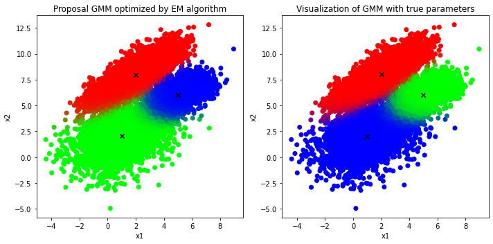
It is clear that the proposal GMM optimized by EM algorithm produces the clusters almost identical to that of the true distribution in which the only difference is the “green” cluster in the proposal GMM is actually the “blue” cluster of the true GMM and vice versa. However, the orderings of those labels do not convey anything as long as a large number of examples is assigned to the correct clusters, which matters the most, and the EM algorithm has delivered an impressive performance in terms of clustering unlabeled dataset into correct classes in this case.
On top of that, the GMM could also describe the uncertainty in deciding clusters for given observations; to be exact, those examples lied at the decision boundaries between clusters tend to have more than two different colors, which means that those data points do not fully commit their weights to any particular cluster. Instead, they partially contribute their weights to multiple clusters at the same time and hence there exists uncertainty for those examples.
Relation between GMM and K-means clustering algorithm
Suppose that each component in the Gaussian-Mixture model has different mean \(\boldsymbol{\mu}_k\) but share the same diagonal covariance matrix govenred by a single parameter \(\sigma^2\). More specifically,
As a result, each component/cluster is expected to be a circular cluster whose radius is equal to that of the other clusters (e.g. because all components shared the same covariance matrix \(\sigma^2\boldsymbol{I}\)), which matches precisely with the assumption of K-means clustering algorithm. That is, each cluster would have different mean but they are equally seperated as well as shared the same circular shape.
Based on that, the density of a data point in a particular cluster \(k\) could be expressed as:
Given the fact that \(k \sim p(k) = \pi_k\), the complete-data log likelihood function could be written as:
Next, in order to apply the EM algorithm as a means to maximize the marginal likelihood of \(\mathbf{X}\), which is \(f(\mathbf{X} = \mathbf{x}|\boldsymbol{\mu}, \sigma^2\boldsymbol{I})\), it remains to evaluate the E-step and M-step to obtain the maximal value of Equation \(\text{(10)}\) while keeping the parameter \(\sigma^2\) fixed.
- E-step:
Recall that the conditional distribution of \(k\) given data \(\mathbf{x}_i\) and previously obtained parameters of interest \(\{\boldsymbol{\mu}^{(t-1)}, \sigma^2, \boldsymbol{\pi}^{(t-1)}\}\) can be obtained easily using the Bayes theorem. That is,
which is of the form of Equation \(\text{(8)}\) except the fact that the formula of \(f(\mathbf{x}_i|\boldsymbol{\mu}_c^{(t-1)}, \sigma^2)\) is replaced by Equation \(\text{(9)}\). Therefore, \(Q(\theta_t, \theta_{t-1})\) should be:
where
- M-step:
Computing the gradient of Equation \(\text{(11)}\) with respect to \(\boldsymbol{\mu}^{(t)}_k\) yields:
For the case of \(\pi_k^{(t)}\), one could introduce a Larange Multiplier term \(\lambda(1 - \sum_k^K \pi_k^{(t)})\) into \(Q(\boldsymbol{\theta}_t, \boldsymbol{\theta}_{t-1})\) so that it becomes:
\(\Rightarrow\) Setting the derivative of Equation \(\text{(14)}\) with respect to \(\pi_k^{(t)}\) to 0 and solving for \(\pi_k^{(t)}\) yields:
It is clear that both Equations \(\text{(13)}\) & \(\text{(15)}\) have the exact same form of Equations \(\text{(3)}\) & \(\text{(7)}\) respectively, and if \(\sigma^2 \to 0\) (e.g. assuming the data point has no variation around its mean), Equation \(\text{(11)}\) becomes:
Knowing that,
\(\Rightarrow\) In the denominator of Equation \(\text{(11)}\), most of the terms for which \(||\mathbf{x}_i - \boldsymbol{\mu}_c||^2\) is large will go to 0 more rapid compared to the term with small magnitude of \(||\mathbf{x}_i - \boldsymbol{\mu}_k||^2\) (presumably \(||\mathbf{x}_i - \boldsymbol{\mu}_k||^2\) is the smallest among other similar terms) since \(\underset{x \to 0}{lim}\space exp(\frac{-100}{x})\) should go to 0 faster than \(\underset{x \to 0}{lim}\space exp(\frac{-1}{x})\).
As a result, \(\gamma_i(k) \to 1\) because the remaining term in both the numerator and denominator is \(\pi_k exp(-\frac{||\mathbf{x}_i - \boldsymbol{\mu}_k ||^2}{2\sigma^2})\), which means that the data point \(\mathbf{x}_i\) is fully contributed to the cluster \(k\) (e.g. \(\gamma_i(c) = 0, \space \forall c \neq k\)) and thus this is equivalently to hard assignment of data points to clusters. To wrap this up, the update formula for \(\boldsymbol{\mu}_k\) and \(\pi_k\) now becomes:
- Stopping criterion:
- There are two possible ways to stop updating parameters when they are already optimal based on given data:
- Assessing whether the difference between the values of marginal likelihood function is less than a certain threshold \(\epsilon\). That is,
$$|L(\boldsymbol{\theta}_t|\mathbf{X}) - L(\boldsymbol{\theta}_{t-1}|\mathbf{X})| \leq \epsilon$$ - Validating whether the distance between the old estimated parameters and the new estimated parameters is less than a pre-defined threshold \(\epsilon\) in which the measurement of distance could be norm, absolute, … depending on the property of those parameters. Specifically,
$$d(\boldsymbol{\theta}_t, \boldsymbol{\theta}_{t-1}) \leq \epsilon$$
- There are two possible ways to stop updating parameters when they are already optimal based on given data:
\(\star\) It is worth mentioning that the solution for updating parameters of GMM with isotropic covariance assumption for every component governed by the parameter \(\sigma^2\), where \(\sigma^2 \to 0\), matches exactly to the solution of updating the centroid at iteration t of K-Means algorithm, which recomputes the centroid based on all data points assigned to the old centroid in the previous iteration. For the case of updating the distribution of a cluster, it is nothing but the total number of points in that cluster divided by the total number of data points for all clusters. Most notably, if \(\sigma^2 \to 0\) is applied to the expected complete-data log likelihood function (e.g. Equation \(\text{(12)}\)), it can be rewritten as:
where,
\(\hskip{4em} r_i(k) =
\begin{cases}
1, \text{ iff } k = \underset{j}{argmin}||\mathbf{x}_i - \boldsymbol{\mu}_j||^2 \\
0, \text{ otherwise}
\end{cases}\)
In Equation \(\text{(18)}\), the mixing coefficients {\(\pi_k\)} have been discarded due to the fact that they are no longer play an important role in maximizing the expected complete-data log likelihood function since the solution of these mixing coefficients is nothing but the fraction of data points assigned to the cluster \(k\) and thereby the value is only from 0 to 1, which would not make any significant impact to Equation \(\text{(18)}\). Also notice that maximizing Equation \(\text{(18)}\) is analogous to minimizing the distortion measure J of K-Means algorithm, where J is of the form:
For now, let us apply the GMM with isotropic covariance in which $\sigma^2 \to 0$ in order to cluster the given data points and compare the result to the output of using K-Means algorithm to cluster the same set of points.
GMM with isotropic covariances governed by \(\sigma^2\) in which \(\sigma^2 \to 0\)
## Initialize parameters to be estimated
# Here only mu is the parameter of interest, which has been explained above.
# Assuming we want to categorize given data points into 3 clusters
est_mus = np.array([[1, 1], [2, 2], [3, 3]])

prev_theta = {'mu': est_mus}
Define function to compute \(r_i(k)\)
def clustering(data, mus):
    '''
        This function simply assigns the given data points to its corresponding cluster as long as
        the distance between itself and the mean of a cluster is minimal. To be specific, this function is
        a replication of r_i(k) function described above

        Parameters
        ----------

        data: Input data to be clustered

        mus: A dictionary contains the centroids of all clusters

        Returns
        -------
        A vector of cluster numbers in which each cluster number is assigned to the corresponding data point
    '''
    result = np.zeros(data.shape[0])
    for i, x in enumerate(data):
        # Calculate the distance between the examining data point and the centroids
        distances = [np.linalg.norm(mu - x) for mu in mus]
        result[i] = np.argmin(distances) # Assign the examining data point to the closest centroid
    return result
Define function to update \(\boldsymbol{\mu}_k^{(t)}\)
def compute_mu_isotropic_GMM(data_features, data_labels):
    '''
        This function simply recomputes the centroids of all clustered data based on the update formula dervied
        from using EM algorithm

        Parameters
        ----------
        data_features: Input data with its associated features

        data_labels: A vector containing cluster labels for the corresponding data

        Returns
        -------
        New centroids for clusters
    '''
    new_centroids = np.zeros((len(np.unique(data_labels)), data_features.shape[1]))
    for cluster_k in np.unique(data_labels):
        data_cluster = data_features[data_labels == cluster_k, :] # Find all points in kth cluster
        new_centroids[int(cluster_k)] = np.mean(data_cluster, axis=0) # Average the coordinates of selected data points
    return new_centroids
Train the GMM with isotropic covariances
In this context, the norm distance between old estimated parameters and new estimated parameters is chosen as the stopping condition for the training process since it is easier than assessing the difference the values of marginal log likelihood function, which need to take into consideration the 0-division issue because \(\sigma^2 \to 0\) as proposed.
# Compute the current theta (in this case mu is only the parameter of interest) based on previous theta
curr_theta = {'mu': compute_mu_isotropic_GMM(data, clustering(data, prev_theta['mu']))}
epsilon = 1e-4 # Define the threshold for stopping criterion

while(max(np.linalg.norm(curr_theta['mu'] - prev_theta['mu'], axis=1)) > epsilon):
    prev_theta['mu'] = curr_theta['mu']
    data_labels = clustering(data, prev_theta['mu'])
    curr_theta['mu'] = compute_mu_isotropic_GMM(data, data_labels)

# Store the estimated mus of Isotropic GMM or K-Means algorithm for later comaprison with generic GMM
isotropic_gmm_mus = curr_theta['mu'].copy()
print('Estimated mus: {}'.format(curr_theta['mu']))
print('True mus: {}'.format(true_theta['mu']))
Estimated mus: [
[0.65707207 1.92490058]
[2.05463048 8.06354715]
[4.92678007 5.91435595]]
True mus: [
[2 8]
[5 6]
[1 2]]
It seems that the \(\boldsymbol{\mu}\) of the 2nd cluster in estimated solution is somewhat similar to the true \(\boldsymbol{\mu}\) of the 1st cluster and the same thing happens with all other estimated \(\boldsymbol{\mu}\) when comparing with other true \(\boldsymbol{\mu}\). Again, the labels of those clusters do not reflect any insightful information as long as the algorithm is able to cluster those given data points in a way that the distribution of the appoximated clusters is analogous to the distribution of the true clusters.
Visualize the clustering result via GMM with isotropic covariances vs that of K-Means using Scikit-Learn
from sklearn.cluster import KMeans # Import K-Means implementation from Sklearn
## Use estimated mu of GMM with isotrpic covariance assumption to perform clustering
isotropic_gmm_labels = clustering(data, curr_theta['mu'])
isotropic_gmm_labels = isotropic_gmm_labels.astype(int)

## Use K-Means algorithm to perform clustering
kmeans = KMeans(n_clusters=3, random_state=0).fit(data)
k_means_labels = kmeans.labels_
## Assign a color to each data point corresponding to its cluster for isotropic GMM
colors_isotropic_gmm = np.zeros((data.shape[0], len(np.unique(data_labels))))
for i, label in enumerate(isotropic_gmm_labels):
if label == 0:
colors_isotropic_gmm[i, :] = np.array([0, 0, 1])
elif label == 1:
colors_isotropic_gmm[i, :] = np.array([0, 1, 0])
else:
colors_isotropic_gmm[i, :] = np.array([1, 0, 0])
## Assign a color to each data point corresponding to its cluster for K-Means
colors_kmeans = np.zeros((data.shape[0], len(np.unique(data_labels))))
for i, label in enumerate(k_means_labels):
if label == 0:
colors_kmeans[i, :] = np.array([0, 0, 1])
elif label == 1:
colors_kmeans[i, :] = np.array([0, 1, 0])
else:
colors_kmeans[i, :] = np.array([1, 0, 0])
## Visualize the result
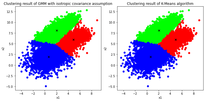
fig, axs = plt.subplots(1, 2, figsize=(10, 5))
axs[0].scatter(x=data[:, 0], y=data[:, 1], c=colors_isotropic_gmm)
axs[0].set_title('Clustering result of GMM with isotropic covariance assumption')
axs[0].scatter(x=curr_theta['mu'][:, 0], y=curr_theta['mu'][:, 1], marker='x', c='black')
axs[1].scatter(x=data[:, 0], y=data[:, 1], c=colors_kmeans)
axs[1].scatter(x=kmeans.cluster_centers_[:, 0], y=kmeans.cluster_centers_[:, 1], marker='x', c='black')
axs[1].set_title('Clustering result of K-Means algorithm')
for ax in axs.flat:
ax.set(xlabel='x1', ylabel='x2')
_ = plt.tight_layout()
print('Esimated mus of GMM with isotropic covariance assumption: {}'.format(curr_theta['mu']))
print('Estimated mus of K-Means algorithm: {}'.format(kmeans.cluster_centers_))
Esimated mus of GMM with isotropic covariance assumption: [
[0.65707207 1.92490058]
[2.05463048 8.06354715]
[4.92678007 5.91435595]]
Estimated mus of K-Means algorithm: [
[0.66422779 1.92626014]
[2.05129912 8.06150275]
[4.93133969 5.92317386]]
Based on the comparison between the solutions of GMM with isotropic covariance assumption & K-Means algorithm, they both seems to match in both quantitative as well as qualitative aspects. To be clear, the estimated means of the GMM & K-Means are almost the same, and when it comes to the visualization, both results are significantly similar leaving only a few minor differences at the boundary between the blue cluster and the green cluster.
Thereby, the term GMM with isotropic covariance assumption and K-Means can now be used interchangbly since they both obtain similar result based on the illustration above.
Visualization of the clustering results of GMM vs K-Means
isotropic_gmm_mus
gmm_mus
colors_gmm
colors_isotropic_gmm
fig, axs = plt.subplots(1, 3, figsize=(15, 5))
axs[0].scatter(x=data[:, 0], y=data[:, 1], c=colors_gmm)
axs[0].scatter(x=gmm_mus[:, 0], y=gmm_mus[:, 1], marker='x', c='black')
axs[0].set_title('Clustering result of GMM optimized by EM algorithm')

axs[1].scatter(x=data[:, 0], y=data[:, 1], c=colors_isotropic_gmm)
axs[1].scatter(x=isotropic_gmm_mus[:, 0], y=isotropic_gmm_mus[:, 1], marker='x', c='black')
axs[1].set_title('Clustering result of K-Means')

axs[2].scatter(x=data[:, 0], y=data[:, 1], c=colors)
axs[2].scatter(x=true_theta['mu'][:, 0], y=true_theta['mu'][:, 1], marker='x', c='black')
axs[2].set_title('Ground truth')

for ax in axs.flat:
    ax.set(xlabel='x1', ylabel='x2')

_ = plt.tight_layout()
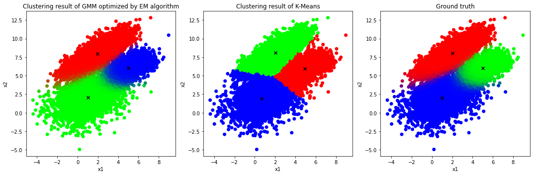
It is clear that the GMM with the help of EM algorithm delivers a better result in comparison with that of K-Means algorithm since K-Means algorithm is a special case of generic GMM and hence the performance of both models is identical if and only if the data is generated from a number of circular clusters with the same radius. Otherwise, generic GMM is a more flexible model in terms of capturing overlapping elliptical clusters with different sizes.
Appendix: Mathematical Concept of EM algorithm
Suppose we are given a dataset \(\mathbf{X} = \{\mathbf{x}_1, \mathbf{x}_2, \cdots, \mathbf{x}_N\}\) in which each observation is assumed to be iid and followed by a particular distribution \(f(\mathbf{x}_i|\boldsymbol{\theta})\), where \(\boldsymbol{\theta}\) is a set of unknown parameters that we wish to optimize in order to maximize the likelihood function \(L(\boldsymbol{\theta}|\mathbf{x}_i)\).
As is often the case that the first attempt is to take the gradient of \(L(\boldsymbol{\theta}|\mathbf{X})\) w.r.t the parameters of interest and solve it to obtain the optimal values for those parameters; however, obtaining the closed-form solution for the parameters of interest via the aforementioned way is not always tractable. For example, given \(L(\boldsymbol{\mu}, \boldsymbol{\Sigma}, \boldsymbol{\pi}|\mathbf{X}) = \pi_1 * \mathcal{N}(\mathbf{X}|\boldsymbol{\mu}_1, \Sigma_1) + \pi_2 * \mathcal{N}(\mathbf{X}|\boldsymbol{\mu}_2, \Sigma_2) + \cdots\) cannot be maximized easily via setting the gradient of this function w.r.t those given parameters to 0 and solve for them. Thereby, one could introduce additional latent variables as a means to obtain the solution in an iterative way while still guaranteeing to get the optimal solution as long as the original likelihood function is convex. Specifically,
Let \(\mathbf{Z} = \{\mathbf{z}_1, \mathbf{z}_2, \cdots, \mathbf{z}_N\}\) be the vector of latent variables associated with all instances in \(\mathbf{X}\). Thus, the complete-data likelihood function can be denoted as \(L(\boldsymbol{\theta}|\mathbf{X}, \mathbf{Z})\), and it is called ‘complete-data’ since \(\mathbf{Z}\) is assumed to be observable resulting in \(L(\boldsymbol{\theta}|\mathbf{X}, \mathbf{Z})\) to be computable. In another words, \(\mathbf{x}_i\) is treated as the observable components of the instance i while \(\mathbf{z}_i\) is the unseen components. The problem now seems getting harder because we actually do not know the form of \(L(\boldsymbol{\theta}|\mathbf{X}, \mathbf{Z})\) and why bother introducing another variable to complicate things more; however, it turns out that is a brilliant way to solve the original problem and please bear with me, things will be more clear once we get the idea of the math behind this algorithm.
For now, there is no doubt that \(L(\boldsymbol{\theta}|\mathbf{X}, \mathbf{Z})\) is a bit ambiguous at a first glance but if the Law of Total Probability is used to express \(L(\boldsymbol{\theta}|\mathbf{X})\) in terms of \(L(\boldsymbol{\theta}|\mathbf{X}, \mathbf{Z})\) , it could be rewritten as:
which means that \(L(\boldsymbol{\theta}|\mathbf{x}_i, \mathbf{z}_i)\) is just a term inside the summation expression of \(L(\boldsymbol{\theta}|\mathbf{x}_i)\)
Furthermore, one can rewrite \(L(\boldsymbol{\theta}|\mathbf{x}_i, \mathbf{z})\) using the Product Rule of Probability as:
As a result, there are many ways to define the complete-data likelihood of \(\mathbf{x}_i\) and \(\mathbf{z}\) using the expressions given above. Next, even though the complete-data likelihood can be obtained, the values of \(\mathbf{z}\) still remain unknown; thus, the most sensible way is to replace those unknown values by their expected value given observable values and most recently obtained parameters. That is,
where \(\boldsymbol{\theta}_{t-1}\) is known and without loss of generality, the expected value of the complete-data log likelihood for all instances with respect to the conditional distribution of \(\mathbf{Z}\) given \(\mathbf{X}\) and \(\boldsymbol{\theta}_{t-1}\) can be depicted as follows:
Most importantly, the reason for taking the expected value of \(L(\boldsymbol{\theta}|\mathbf{X}, \mathbf{Z})\) w.r.t the conditional distribution of \(\mathbf{z}\) given \(\mathbf{x}_i\) and \(\boldsymbol{\theta}\) is the fact that:
and so the log likelihood function of \(\boldsymbol{\theta}\) given \(\mathbf{X}\) is indeed comprised of \(Q(\boldsymbol{\theta}|\boldsymbol{\theta}_{t-1})\)
as well as \(H(p||q)\) is the cross entropy of the distribution q relative to the distribution p.
Considering \(log(f(\mathbf{X}|\boldsymbol{\theta})\) could be expressed as a function of \(\boldsymbol{\theta}\) via Equation \(\text{(20)}\) and thus if \(\boldsymbol{\theta}\) is replaced by \(\boldsymbol{\theta}_{t-1}\), Equation \(\text{(20)}\) would become:
Subtract \(log f(\mathbf{X}|\boldsymbol{\theta}_{t-1})\) from \(log f(\mathbf{X}|\boldsymbol{\theta})\) yields
Consequently, \(Q(\boldsymbol{\theta}|\boldsymbol{\theta}_{t-1}) - Q(\boldsymbol{\theta}_{t-1}|\boldsymbol{\theta}_{t-1})\) is obviously the lowerbound of \(log f(\mathbf{X}|\boldsymbol{\theta}) - log f(\mathbf{X}|\boldsymbol{\theta}_{t-1})\) and thereby improving \(Q(\boldsymbol{\theta}|\boldsymbol{\theta}_{t-1})\) would lead to the increase in \(log f(\mathbf{X}|\boldsymbol{\theta})\) as illustrated by Equation \(\text{(21)}\). In other words, if \(Q(\boldsymbol{\theta}|\boldsymbol{\theta}_{t-1}) - Q(\boldsymbol{\theta}_{t-1}|\boldsymbol{\theta}_{t-1}) > 0\), then \(log f(\mathbf{X}|\boldsymbol{\theta}) - log f(\mathbf{X}|\boldsymbol{\theta}_{t-1}) > 0\), which is equivalently saying that the increase in \(Q(\boldsymbol{\theta}|\boldsymbol{\theta}_{t-1})\) relative to \(Q(\boldsymbol{\theta}_{t-1}|\boldsymbol{\theta}_{t-1})\) would result in the increase in \(log f(\mathbf{X}|\boldsymbol{\theta})\) relative to \(log f(\mathbf{X}|\boldsymbol{\theta}_{t-1})\).
Last but not least, it remains to define the conditional distribution of \(\mathbf{z}\) given \(\mathbf{x}_i\) \(\boldsymbol{\theta}_{t-1}\) as the last piece of unknown quantity in order to evaluate \(Q(\boldsymbol{\theta}|\boldsymbol{\theta}_{t-1})\) and hence maximization of \(Q(\boldsymbol{\theta}|\boldsymbol{\theta}_{t-1})\) becomes feasible as a means to maximize the marginal likelihood function \(L(\boldsymbol{\theta}|\mathbf{X})\). Based on Bayes’ theorem, one could express \(f(\mathbf{z}_i|\mathbf{x}_i, \boldsymbol{\theta}_{t-1})\) as follows:
All things considered, the EM algorithm could be summarized within the following steps below:
- E-Step:
- Define the complete-data log likelihood function for a single observation \(\mathbf{x}\), which is \(l(\boldsymbol{\theta}|\mathbf{x}, \mathbf{z})\)
- Define the conditional distribution of latent variables \(\mathbf{z}\) given observable variables \(\mathbf{x}\) and parameters of interest obtained recently \(\boldsymbol{\theta}_{t-1}\), which essentially is \(f(\mathbf{z}|\mathbf{x}, \boldsymbol{\theta}_{t-1})\)
- Evaluate \(Q(\boldsymbol{\theta}|\boldsymbol{\theta}_{t-1} = E_{\boldsymbol{\theta}_{t-1}}[l(\boldsymbol{\theta}|\mathbf{X}, \mathbf{Z}) | \mathbf{X}]\)
- M-Step:
- Setting the gradient of \(Q(\boldsymbol{\theta}|\boldsymbol{\theta}_{t-1})\) with respect to parameters of interest \(\boldsymbol{\theta}\) to 0 and solving for \(\boldsymbol{\theta}\)
- Repeat the aforementioned 2 steps above until either one of those conditions satisfied:
- \[|l(\boldsymbol{\theta}|\mathbf{X}) - l(\boldsymbol{\theta}_{t-1}|\mathbf{X})| \leq \epsilon\]
- \(d(\boldsymbol{\theta}, \boldsymbol{\theta}_{t-1}) \leq \epsilon\)
where \(\epsilon\) is simply a predefined threshold and \(d(\boldsymbol{\theta}, \boldsymbol{\theta}_{t-1})\) is a kind of distance between \(\boldsymbol{\theta}\) and \(\boldsymbol{\theta}_{t-1}\) decided by practitioners.
References
[1] Christopher M. Bishop. Pattern Recognition and Machine Learning, Section 9.3.2, Chapter 9.
[2] D.P. Kroese and J.C.C. Chan. Statistical Modeling and Computation, Section 6.6, Chapter 6.