Gaussian Processes

Introduction

In supervised learning approach, choosing a parametric model (e.g. linear reg, logistic reg and so on) is the most preferable way to do the predictive analysis, since the mathematical derivation for finding the optimal parameters \(\boldsymbol\theta\) via either point estimation \(\boldsymbol{\hat\theta}\) or Maximum Likelihood Estimation (MLE) \(p(\mathbf{y}|\mathbf{X}, \boldsymbol\theta)\) in the sense of statistics is somehow attractive and straightforward.

However, when it comes to data with high complexity (non-linear relationships in data), a parametric model must increase its number of parameters in order to explain the data reasonably well, which requires a large amount of computational resource to train the grand-scale model.

To tackle this issue, one of the most renowned solutions is to use non-parametric methods, where the model’s complexity can automatically adjust based on the given dataset without sacrificing huge computational power for more parameters to capture the complexity of data.

A typical example would be the Gaussian Processes (GPs). GPs is a non-parametric method since it, instead of inferring a distribution over the parameters, infers a distribution over the functions directly. A Gaussian process defines a prior over functions and then converts into a posterior over functions after it observes some function values => Inference of continuous function values in this context is known as GPs regression, but GPs can also be used in classification.

Gaussian Processes Definition

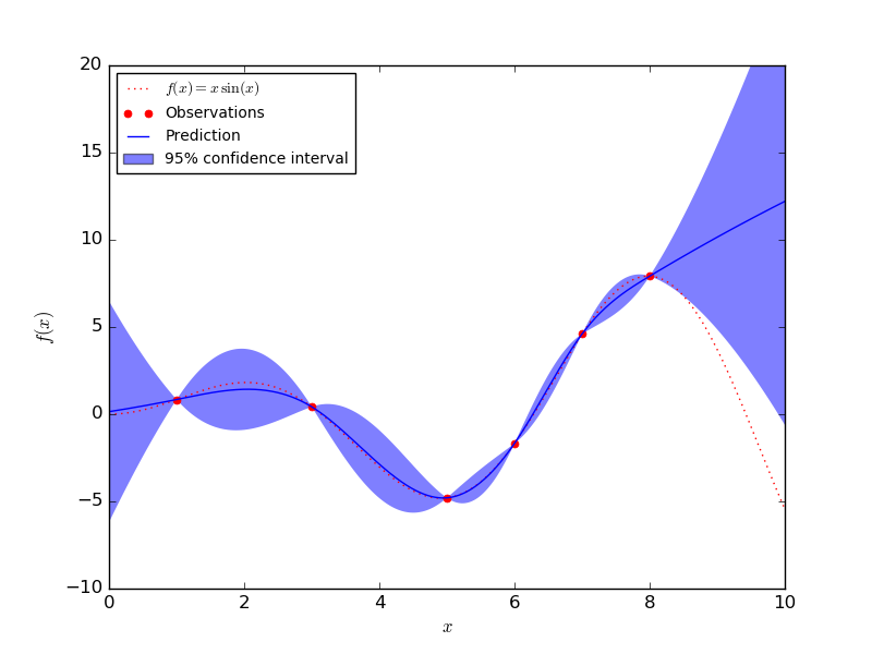
A Gaussian Processes (GPs) is a non-parametric and probabilistic model for nonlinear relationships. The more data arrives the more flexibility and complexity the model could be when using GPs. The figure below illustrates an example of using GPs as a regression method to approximate function \(f(x) = xsin(x)\).

GPs assumes that any point \(\mathbf{x}\in \mathbb{R}^d\) is assigned a random variable \(f(\mathbf{x})\) and the joint distribution of a finute number of these variables \(p(f(\mathbf{x}_1),..., f(\mathbf{x}_N))\) is itself a Gaussian distribution:

which is similar to:

where,

in which \(\mathbf{K}_{1}\) is a kernel block matrix contains 2-input kernel values for all combinations of \(x_1\) to \(x_i\) with \(i < N\)

This representation of a GPs is similar to a multivariate normal distribution. Instead of displaying samples drawn from this distribution as a vector containing N elements, it could be represented as a vector containing 2 elements such that \(1^{st}\) element has M values and \(2^{nd}\) element has Q values, where M + Q = N

where,

In Equation \(\text{(1)}\), the covariance of the distribution is defined by the kernel function \(\mathbf{K_{ij}} = k(\mathbf{x}_i, \mathbf{x}_j)\) (it could be squared exponential kernel or linear kernel and so on). Thus, the shape of the function (e.g. smoothness) is defined by \(\mathbf{K}\).

Given a set of data \(\mathbf{D} = \{(\mathbf{x}_i, y_i)\}\) or \(\mathbf{X}, \mathbf{y}\) and ultilizing the definition of prior GPs \(p(\mathbf{f}|\mathbf{X})\) in combination with the assumption of modeling the target/outcome \(\mathbf{y}\) in terms of \(\mathbf{f}\) discussed in \(\textbf{Part II}\), we can then integrate those information altogether so as to derive the predictive distribution of GPs \(p(\mathbf{f}^*|\mathbf{X}^*, \mathbf{X}, \mathbf{y})\) to make prediction \(\mathbf{f}^{*}\) given new input \(\mathbf{X}^{*}\). The coming up steps are affiliated with the inference of posterior predictive distribution of GPs,

Part I

Since we have already assumed our data follows the Gaussian Processes assumption, which means not only the prior follows GPs model (\(p(\mathbf{f}) \sim \mathcal{N}(0, \mathbf{K}_f)\)) but the unseen data must also obey the GPs model that inherits the form analogous to the prior GPs structure and belongs to Gaussian family (\(p(\mathbf{f}^*) \sim \mathcal{N}(0, \mathbf{K}_f^*)\)). Thus, the joint distribution of \(p(\mathbf{f}, \mathbf{f}^*)\) would also be a Gaussian that is conjugate to its prior, to be specific, it is a multivariate normal distribution (jointly normal distributed) which can be represented as a bivariate normal distribution of 2 vectors \(\mathbf{f}\) & \(\mathbf{f}^*\) as shown in Equation \(\text{(2)}\). Consequently, the result is identified as follows

Assuming that the mean \(\boldsymbol\mu\) is set to 0 for simplicity. The covariance matrix \(\mathbf{K}_{f}\) of \(\mathbf{f}\) is defined as \(Cov(\mathbf{X}, \mathbf{X})\) computing by input data \(\mathbf{X}\). By the same token, \(\mathbf{K}_{*}\) is assigned to \(Cov(\mathbf{X}, \mathbf{X}^*)\) and \(\mathbf{K}_{**} = Cov(\mathbf{X}^*, \mathbf{X}^*)\).

\(\longrightarrow\) \(p(\mathbf{f}^*|\mathbf{X}^*,\mathbf{X},\mathbf{f})\) can be derived easily since it is the conditional distribution of the joint normal distribution \(p(\mathbf{f}, \mathbf{f}^*| \mathbf{X}, \mathbf{X}^*)\) with its mean \(\boldsymbol{\mu}_{\mathbf{f}^{*}|\mathbf{f}}\) and covariance \(\boldsymbol{\Sigma}_{\mathbf{f}^*|\mathbf{f}}\) can be defined according to the result \(\mathbf{(2.115)}\) from textbook \(\textbf{Pattern Recognition and Machine Learning}^{[1]}\),

Part II

In reality, the target/outcome \(\mathbf{y}\) of the data is commonly modeled by a mathematical formula \(\mathbf{f}(\mathbf{X})\), which is an interpretable part, including an unexplained part or noise factor modelled as a Gaussian distribution \(\boldsymbol\epsilon \sim \mathcal{N}(0, \sigma^2_y\mathbf{I})\), and that is also a reasonable assumption and straightforward when combining the GPs and the noise altogether. In general, the outcome of the data is represented as \(\mathbf{y} = \mathbf{f}(\mathbf{X}) + \boldsymbol\epsilon\), which is equivalent to put the definition of prior GPs of \(p(\mathbf{f}|\mathbf{X})\) and the presence of \(\boldsymbol\epsilon\) together. Hence the GPs posterior \(p(\mathbf{y}|\mathbf{f}, \mathbf{X})\) could be interpreted as follows,

or

According to \(\underbrace{\text{Part II}}\) in Equation \(\text{(3)}\),

where,

\(\implies p(\mathbf{y}|\mathbf{X}, \mathbf{f})p(\mathbf{f}) \sim \mathcal{N}(\mathbf{u}, \boldsymbol{\Lambda}) \tag{6}\)

Part III

Regarding the results have been derived in \(\textbf{Part I}\) and \(\textbf{Part II}\), which are both belong to Gaussian distribution family; therefore, it is obvious that the product of those is also a Normal distribution that has the following form

where,

The derivation of Equations \(\text{(7)}\) & \(\text{(8)}\) requires plenty of complicated linear algebra works to accomplish, so it is better not to mention in this article, but if the curiosity completely takes control of yourself, \(\textbf{Technical Introduction of GPs Regression}^{[2]}\) describes every step to come up with \(\textbf{Part III}\) results. However, the idea of proof is quite straightforward, consider the product of two Gaussian distributions in 1D case:

Let \(X|Y \sim \mathcal{N}(\mu_{x|y}, \sigma^2_{x|y})\) and \(Y \sim \mathcal{N}(\mu_y, \sigma^2_y)\), where \(\mu_{x|y} = ay\) is a function of \(y\) similar to \(\boldsymbol{\mu}_\mathbf{f^*|f}\) is also a function of \(\mathbf{f}\) and \(X|Y\) & \(Y\) could be thought of \(p(\mathbf{f}^*|\mathbf{f}, \mathbf{X}, \mathbf{X}^*)\) & \(p(\mathbf{f})\) respectively. Hence, the marginal distribution of \(X\) is the integral of the product of these two distributions w.r.t \(Y\). Specifically define,

Simplify \(BA^{-1}\) & \(A^{-1}\) and map

The result should be accordance to \(\text{(7)}\) and \(\text{(8)}\).

Implementation

''' Import all necessary packages for later use '''
%matplotlib notebook
import sys
import numpy as np
import matplotlib
import matplotlib.pyplot as plt
from matplotlib import cm # Colormaps
import matplotlib.gridspec as gridspec
from mpl_toolkits.axes_grid1 import make_axes_locatable
import seaborn as sns
from matplotlib import cm
from mpl_toolkits.mplot3d import Axes3D
sns.set_style('darkgrid')
np.random.seed(42)

Regarding the kernel function used to evaluate the covariance for a pair of observations, the exponential kernel is carried out for this implementation, also known as Gaussian kernel or RBF kernel:

\(\kappa(\mathbf{x}_i,\mathbf{x}_j) = \sigma_f^2 \exp(-\frac{1}{2l^2} (\mathbf{x}_i - \mathbf{x}_j)^T (\mathbf{x}_i - \mathbf{x}_j))\tag{9}\)

The length parameter \(l\) controls the smoothness of the function and \(\sigma_f\) the vertical variation. For simplicity, we use the same length parameter \(l\) for all input dimensions (isotropic kernel).

def kernel(X1, X2, l=1.0, sigma_f=1.0):
''' 
    Isotropic squared exponential kernel. Computes a covariance matrix from points in X1 and X2.
    
    Parameters
    ----------
    X1: Array of m points (m x d)
    
    X2: Array of q points (q x d)
    
    Return
    ------
    cov_s: a NumPy array
        Covariance matrix (m x q)
    
    Notes
    -----
    1st arg = -1 in reshape means that it lets numpy automatically infer the number of elements for the 1st axis 
    if we specified 1 element for the 2nd axis 
    -> np.sum(X1**2, 1).reshape(-1, 1) returns an array with the shape of (m, 1)
        where n is the number of observations in X1
        
    X1^2 with shape (m, 1) + X2^2 with (q, ) will return a mxq matrix whose row entries = row element in X1^2 + each element in X2^2

'''
sqdist = np.sum(X1**2, 1).reshape(-1, 1) + np.sum(X2**2, 1) - 2 * np.dot(X1, X2.T)
return sigma_f**2 * np.exp(-0.5 / l**2 * sqdist)

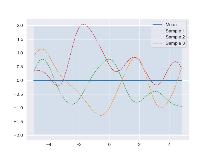
Define Prior: p(f|X)

Asssume that the prior over functions with mean zero and covariance matrix calculated by the RBF kernel with \(l = 1\) and \(\sigma_f = 1\). The code snippet below is an illustration of drawing 3 random sample functions and plots it together with zero mean and 95% confidence interval (computed from the diagonal of covariance matrix).

def plot_gp(mu, cov, X, X_train=None, Y_train=None, samples=[]):
'''
    Plot the distribution of functions drawn from GPs including the mean function with 95% confidence interval
    
    Parameters
    ----------
    mu: a NumPy array
        The mu values of the GPs distribution (could be prior or posterior predictive)
    cov: a NumPy array
        The covariance matrix of the GPs distribution (could be prior or posterior predictive)
    X: a NumPy array
        An array of inputs used to compute cov matrix and represented along x-axis
    X_train: a NumPy array
        An array of training inputs used to compute cov matrix 
        and combined with its outputs from posterior predictive dist 
        to form data points with red cross notation on the graph
    Y_train: a NumPy array
        An array of training outputs corresponds with X_train
    samples: a NumPy array
        An array contains sample functions drawn from prior or posterior predictive distribution
    
    Return
    ------
    NoneType
'''
X = X.ravel()
mu = mu.ravel()
uncertainty = 1.96 * np.sqrt(np.diag(cov))

plt.fill_between(X, mu + uncertainty, mu - uncertainty, alpha=0.1)
plt.plot(X, mu, label='Mean')
for i, sample in enumerate(samples):
    plt.plot(X, sample, lw=1, ls='--', label=f'Sample {i+1}')
if X_train is not None:
    plt.plot(X_train, Y_train, 'rx')
plt.legend()

''' Draw sample from prior GPs '''
# Finite number of points
X = np.arange(-5, 5, 0.2).reshape(-1, 1)

# Mean and covariance of the prior
mu = np.zeros(X.shape[0])
cov = kernel(X, X)

# Draw three samples from the prior
samples = np.random.multivariate_normal(mu, cov, 3)

# Plot GPs mean, confidence interval and samples 
plot_gp(mu, cov, X, samples=samples)

Define Posterior Predictive: \(p(f^*|X^*, X, y)\)

from numpy.linalg import inv
def posterior_predictive(X_test, X_train, Y_train, l=1.0, sigma_f=1.0, sigma_y=1e-8):
    '''
        Compute the mean and the covariance of posterior predictive distribution based on given data including the inference for testing data
        
        Parameters
        ----------
        X_test: a NumPy array
            Input of testing data
        X_train: a NumPy array
            Input of training data
        Y_train: a NumPy array
            Output of training data
        l, sigma_f: float number, default=1.0, 1.0
            Hyper parameter of squared exponential kernel function
        sigma_y: float number, default=1e-8
            Noise assumption parameter the output data
        
        Return
        ------
        mu_s: a NumPy array
            The mean of posterior predictive distribution
        cov_s: a NumPy array
            The covariance matrix of posterior predictive distribution
    '''
    K = kernel(X_train, X_train, l, sigma_f) + sigma_y**2 * np.eye(len(X_train))
    K_s = kernel(X_train, X_test, l, sigma_f)
    K_ss = kernel(X_test, X_test, l, sigma_f) + 1e-8 * np.eye(len(X_test))
    K_inv = inv(K)
    
    # Equation (7)
    mu_s = K_s.T.dot(K_inv).dot(Y_train)

    # Equation (8)
    cov_s = K_ss - K_s.T.dot(K_inv).dot(K_s)
    return mu_s, cov_s

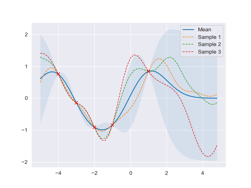
Prediction with noise-free assumption

According to the derivation of posterior predictive distribution, if the inference is carried out based on those given assumption, the output of the data would have the form \(y_i = f(\mathbf{x}_i) + \epsilon\), or generally \(\mathbf{y} = \mathbf{f(X)} + \boldsymbol\epsilon\).

It, therefore, is clear that the model is already taken noise into account, which is distinct from the noise-free model \(\mathbf{y} = \mathbf{f}(\mathbf{X})\), that is regardless of the number of attempts trying to predict the output \(\mathbf{y}\) with the same input \(\mathbf{X}\) the result would still be the same -> no variation (noise) for the outputs with the same input (e.g. 1st time: \(f(5) = 10.1\), 2nd time: \(f(5) = 10.1\), 3rd time: \(f(5) = 10.1)\)), which is far removed from the outputs having noise included (e.g. 1st time: \(f(5) = 10.1\), 2nd time: \(f(5) = 10.5\), 3rd time: \(f(5) = 9.8)\)).

Hence, in order to achieve the noise-free model \(\mathbf{y} \sim \mathcal{N}(\mathbf{f}, 0)\), we can use a simple trick, that is set the variance of \(\mathbf{y}\) \(\sigma^2_y\) to an extremely small number towards 0 (\(\sigma^2_y \rightarrow 0\)), say 1e-8. By doing so, even tons of tries to generate a large number of outcome values \(y_i\) having the same input \(x_i\), the results would still be significantly identical to each other (e.g. 9.9999998, 9.99999999,…) since the variability described by \(\sigma^2_y\) is almost 0.

''' Derive predictive model with noise-free assumption '''
X_train = np.array([-4, -3, -2, -1, 1]).reshape(-1, 1)
Y_train = np.sin(X_train)
X_test = np.arange(-5, 5, 0.2).reshape(-1, 1)

# Compute mean and covariance of the posterior predictive distribution
mu_s, cov_s = posterior_predictive(X_test, X_train, Y_train)

# Draw three samples from the posterior predictive distribution
''' In this case, the (N, 1) array mu_s is flattened before passing into np.random.multivariate_normal 
        since its requirement for the mean argument must be a (N, ) array
'''
samples = np.random.multivariate_normal(mu_s.ravel(), cov_s, 3)

# Plot the result
plt.clf()
plot_gp(mu_s, cov_s, X_test, X_train=X_train, Y_train=Y_train, samples=samples)

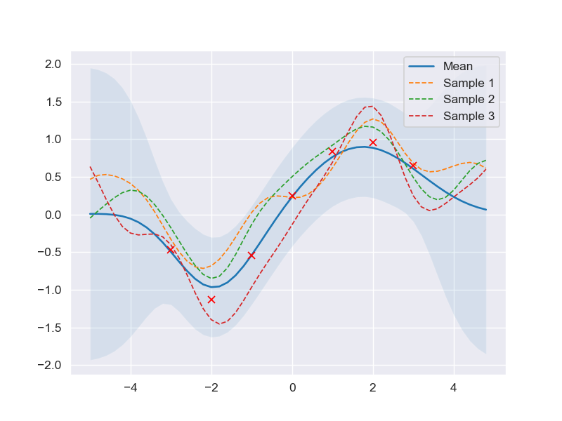
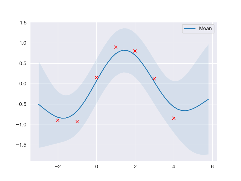
Prediction with noise assumption (normal assumption)

When it comes to the practical scenario, there is no mathematical model that can capture all the complexity as well as the variation of the data (a.k.a be able to predict the outcome exactly 100%).

That is why introducing the uncertainty to the mathematical model is necessary in order to have a complete picture about the possible values of prediction compared to the real-world results, to be precise, the predictive equation should be

''' Derive predictive model with noise assumption '''
noise = 0.4
# Noisy training data
X_train = np.arange(-3, 4, 1).reshape(-1, 1)
Y_train = np.sin(X_train) + noise * np.random.randn(*X_train.shape)
X_test = np.arange(-5, 5, 0.2).reshape(-1, 1)

# Compute mean and covariance of the posterior predictive distribution
mu_s, cov_s = posterior_predictive(X_test, X_train, Y_train, sigma_y=noise)

samples = np.random.multivariate_normal(mu_s.ravel(), cov_s, 3)
plot_gp(mu_s, cov_s, X_test, X_train=X_train, Y_train=Y_train, samples=samples)

Optimizing kernel hyperparameters

Before getting straight to the point, let us examine the the effect of kernel parameters \(l\) and \(\sigma_f\) as well as \(\sigma_y\) in order to decide whether it is necessary to optimize these parameters or not.

''' Try building different predictive models with different hyperparameters' values of the RBF kernel '''
X_train = np.arange(-2, 5, 1).reshape(-1, 1)

X_test = np.arange(-3, 6, 0.2).reshape(-1, 1)
params = [
    (3.0, 1.0, 0.5),
    (0.3, 1.0, 0.5),
    (1.0, 3.0, 0.5),
    (1.0, 0.3, 0.5),
    (1.0, 1.0, 1.5),
    (1.0, 1.0, 0.1)
]

plt.figure(figsize=(9, 5))

for i, (l, sigma_f, sigma_y) in enumerate(params):
    Y_train = np.sin(X_train) + sigma_y * np.random.randn(*X_train.shape)
    mu_s, cov_s = posterior_predictive(X_test, X_train, Y_train, l=l, sigma_f=sigma_f, sigma_y=sigma_y)
    plt.subplot(3, 2, i + 1)
    plt.title(f'l = {l}, sigma_f = {sigma_f}, sigma_y = {sigma_y}')
    plt.tight_layout()
    plot_gp(mu_s, cov_s, X_test, X_train=X_train, Y_train=Y_train)

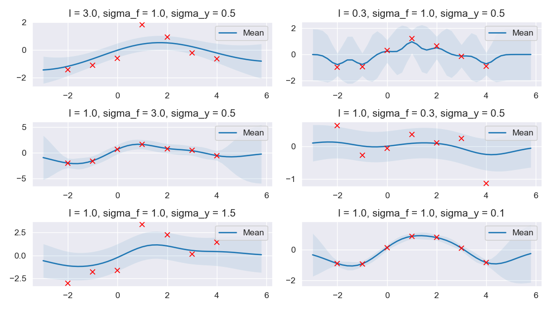Regarding the figure above,

1. The \(1^{st}\) 2 subplots shows that the higher value \(l\) is, the smoother function would be and the lower value \(l\) can make the function more wiggly.

2. Two subplots of the \(2^{nd}\) row illustrates that \(\sigma_f\) controls the vertical variation of the function drawn from GPs, that is higher value of \(\sigma_f\) would make the function captures all the training data, thus small confidence interval in the training data region and wide confidence interval outside the area where training data exists; thus, by choosing the lower value of \(\sigma_f\), this would lead to a function with coaser approximation (wide confidence interval) as shown in the \(2^{nd}\) subplot from the \(2^{nd}\) row.

3. About the last 2 subplots, higher variation in data leads to coaser approximation in the \(1^{st}\) subplot which can avoid overfitting compared to lower value of \(\sigma_y\) that causes function drawn from GPs fits the training data too well even if there might be some training data which are considered as noises.

In a nutshell, better parameters values opted for the covariance kernel would yield a better result in regression.

As already discussed about the joint distribution of GPs \(p(\mathbf{f},\mathbf{f}^*)\), the noise variation has been introduced to the variable \(\mathbf{f}\); hence, for the ease of discrimination, treat \(p(\mathbf{f},\mathbf{f}^*)\) (without \(\sigma_y^2\)) and \(p(\mathbf{y},\mathbf{f}^*)\) (with \(\sigma_y^2\)) are the both the joint normal distribution which have the same formula with only the diagonal entries inside the covariance matrix are distinct. Since \(p(\mathbf{y}, \mathbf{f}^*)\) is the jointly Normal distribution relatively analogous to Equation \(\text{(2)}\), the marginal distribution of \(p(\mathbf{y})\) or \(p(\mathbf{y}|\mathbf{X})\), therefore, can be expressed as

\(\implies\) Set of parameters including \(l\), \(\sigma_f\), and \(\sigma_y\) can be tunned by making use of the marginal distribution \(p(\mathbf{y})\), to be precise, \(p(\mathbf{y}|\mathbf{X})\) can be represented as the cost function of \(l\), \(\sigma_f\), and \(\sigma_y\) by taking the negative logarithm of its PDF:

from numpy.linalg import cholesky, det, lstsq
from scipy.optimize import minimize

def neg_ll_function(X_train, Y_train, noise):
    '''
        Compute the log-likelihood function of the marginal distribution function p(y|X)
        
        Parameters
        ----------
        X_train: a NumPy array with MxD dimension
            Input of training data
        
        Y_train: a NumPy array with Mx1 dimension
            Output of training data
        
        noise: float number
            Noise assumption {sigma_y} for the target/output of the data (y = f(x) + noise)
            which is also associated in the calculation of covariance matrix (discussed in prediction with noise assumption section)
        
        theta: a NumPy array with 2x1 dimension
            An array containing l value & sigma_f value
            
        Return
        ------
        Returns minimization objective (Equation 6)
    '''
    def equation_6(theta):
        K = kernel(X_train, X_train, l=theta[0], sigma_f=theta[1]) + (noise ** 2 * np.eye(len(Y_train)))
        return  0.5 * np.log(det(K)) + \
                0.5 * Y_train.T.dot(inv(K).dot(Y_train)) + \
                0.5 * len(Y_train) * np.log(2 * np.pi)
    
    return equation_6

noise = 0.4
# Minimize the negative log-likelihood w.r.t. parameters l and sigma_f.
# We should actually run the minimization several times with different # of initializations to avoid local minima but this is skipped here for simplicity. 
res = minimize(neg_ll_function(X_train, Y_train, noise), \
               [1, 1], \
               bounds=((1e-5, None), (1e-5, None)), \
               method='L-BFGS-B')

# Store the optimization results in global variables so that we can compare it later with the results from other implementations. 
l_opt, sigma_f_opt = res.x

# Compute the prosterior predictive statistics with optimized kernel parameters and plot the results 
mu_s, cov_s = posterior_predictive(X_test, X_train, Y_train, l=l_opt, sigma_f=sigma_f_opt, sigma_y=noise)
plot_gp(mu_s, cov_s, X_test, X_train=X_train, Y_train=Y_train)

Higher dimensions implementation

In this section, higher-dimension input data (2D input data expanded in x-y plane in this case) will be used as the input for GPs to fit the outcome that is actually came from a sine wave originating at 0 with noise added.

def plot_gp_2D(gx, gy, mu, X_train, Y_train, title, i):
    '''
        Plot a regression surface derived from GPs including scattered data points 
        where 2D input data is displayed in x-y plane & the output values is mapped to z plane
        
        Parameters
        ----------
        gx, gy: NumPy arrays
            Grid of x & y testing inputs generated from np.meshgrid (X, Y arguments for ax.plot_surface)
        
        mu: a NumPy array
            Grid of output/expected values derived from GPs whose inputs are gx, gy (Z argument for ax.plot_surface)
            
        X_train: a NumPy array
            An array of training inputs where each row entry contains x & y values
        
        Y_train: a NumPy array
            An array of training outputs which is corresponding to X_train array
        
        title: string
            Plot title
        
        i: integer
            An integer determines which subplot should be activated
            
        Return
        ------
        None
            
    '''
    ax = plt.gcf().add_subplot(1, 2, i, projection='3d')
    ax.plot_surface(gx, gy, mu.reshape(gx.shape), cmap=cm.coolwarm, linewidth=0, alpha=0.2, antialiased=False)
    ax.scatter(X_train[:,0], X_train[:,1], Y_train, c=Y_train, cmap=cm.coolwarm)
    ax.set_title(title)

''' Build predictive model for multi-dimensional data '''
noise_2D = 0.1

# Testing x & y inputs 
rx, ry = np.arange(-5, 5, 0.3), np.arange(-5, 5, 0.3)
# Create meshgrid for rx & ry so that all pairs of every x in rx & every y in ry are established
gx, gy = np.meshgrid(rx, rx)
# Combine gx, gy generated from meshgrid to a vector whose element is consisted of pair of x & y values
X_2D_test = np.c_[gx.ravel(), gy.ravel()]

# Generate training data
X_2D_train = np.random.uniform(-4, 4, (100, 2))
Y_2D_train = np.sin(0.5 * np.linalg.norm(X_2D_train, axis=1)) + \
             noise_2D * np.random.randn(len(X_2D_train))

plt.figure(figsize=(14,7))

mu_s, _ = posterior_predictive(X_2D_test, X_2D_train, Y_2D_train, sigma_y=noise_2D)
plot_gp_2D(gx, gy, mu_s, X_2D_train, Y_2D_train, 
           f'Before parameter optimization: l={1.00} sigma_f={1.00}', 1)

res = minimize(neg_ll_function(X_2D_train, Y_2D_train, noise_2D), [1, 1], 
               bounds=((1e-5, None), (1e-5, None)),
               method='L-BFGS-B')

mu_s, _ = posterior_predictive(X_2D_test, X_2D_train, Y_2D_train, *res.x, sigma_y=noise_2D)
plot_gp_2D(gx, gy, mu_s, X_2D_train, Y_2D_train,
           f'After parameter optimization: l={res.x[0]:.2f} sigma_f={res.x[1]:.2f}', 2)

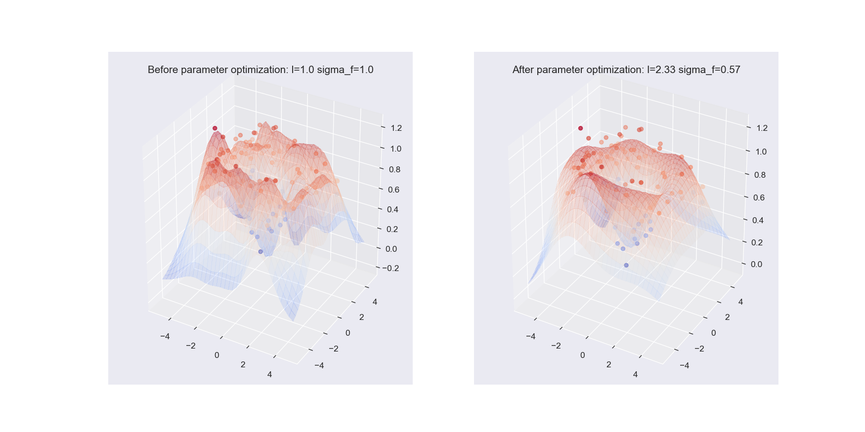
Notice that, the approximation of sine wave function based on GPs after optimizing the kernel parameters is way more better (closer to the true sine function) compared to the regression result before applying parameter optimization.

Reference

[1] Christopher M. Bishop. Pattern Recognition and Machine Learning, Chapter 6.
[2] A Technical Introduction to Gaussian Processes Regression
[3] Gaussian Processes - Krasserm
[4] Gaussian Processes for Dummies - Katbailey